Trusted AI: The Science of Monotonicity in Neural Networks
In part 2 of this series, I take a deep dive into the data science that drives monotonicity and palatability, qualities that help gain trust in AI


Welcome to Part 2 of my exploration of monotonicity in neural networks. In this blog I’ll get into some of the data science techniques we’ve developed at FICO to ensure monotonicity in neural networks. Monotonicity is essential to build trust and auditability in decision models used in regulated industries such as lending, where fair, unbiased decisioning is the top priority for all parties involved: lenders, customers and regulators.
Monotonicity Recap
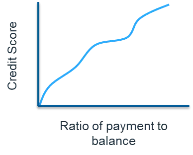
Here’s a snippet from Part 1 of this series, to provide some context: In an analytic model, a monotonic relationship occurs when an input value is increased and the output value either only increases (positively constrained) or only decreases (negatively constrained), and vice versa. For example, if the ratio of payment to balance owed on a loan or credit card increases, we would expect that the credit risk score should improve (lower risk of default). Figure 1 shows a positively constrained monotonic relationship between these two variables.
FICO’s innovation in explainable neural network technology imposes monotonicity requirements on inputs and outputs. We accomplish this by putting additional constraints on the training of the neural networks, guaranteeing a computationally efficient (and convergent) solution with the desired monotonicity constraints. Our approach, described below, leverages the same gradient descent-based optimization approach for training the neural network, and as such it also guarantees the best fit model.
Setting Model Constraints Properly
The training of a monotonic neural network requires us to specify a polarity value for all the nodes, which constrains the relationship between the changes in the values of the two connected nodes. Polarity values can be +1, -1 or 0. The polarity of the output is always set to +1 and all the other polarities are in reference to this polarity. The polarity of the input can be set to +1, -1 or 0 by the users, based on whether they need a positively constrained monotonic relationship, negatively constrained relationship or no constraints in the relationship with the output.
The polarities of the hidden nodes are set as part of the model training. The key aspect is that connections with the same polarities imply that an increase in the value of the first node would yield an increase in the value of the second node, and vice versa. Similarly, the connections with opposite polarities imply that an increase in the value of the first node would yield a decrease in the value of the second node and vice versa.
Figure 2 shows positively constrained relationship between input variable v2, ratio of payment/balance, and output node S. It also shows a negatively constrained relationship between input variable v3, amount owed across all tradelines, and output node S.
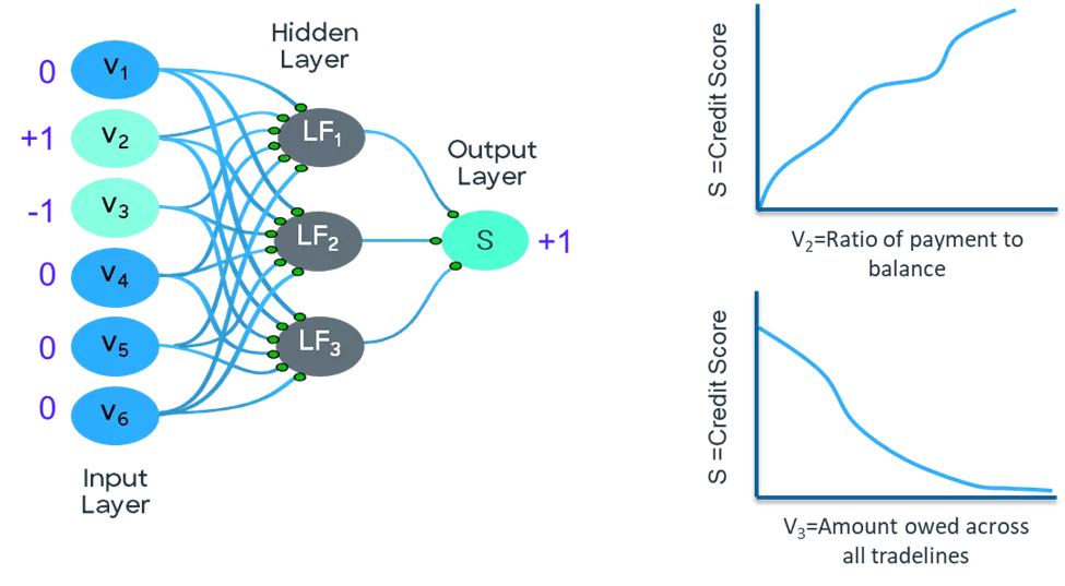
The output is unconstrained with respect to the rest of the input variables. In this example, v2 is payment as proportion of balance, v3 is the amount owed across all tradelines and S is credit risk score. An increase in value of v2 leads to increase in the value of S. On the other hand, an increase in value of v3 reduces the output S due to increased risk of default. Figure 2 shows how the initial constraints imposed for these two scenarios are set before model training begins.
The Relationship between Model Connections and Constraints
The polarities of the two connected nodes determine the relationship between the changes in the values between the first node and the second node, by constraining the sign of the weight of the connection connecting them. This is shown in Figure 3, such that the cases where the polarities of two connected nodes are same, the weight of the connection connecting them is constrained to be positive. If their polarities are different, the weight of the connection connecting them is constrained to be negative.
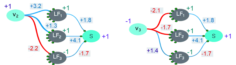
Figure 3: The polarities of each node must be monitored throughout optimization iterations
For example, since polarities of both v2 and LF1 are positive, the weight of the connection is shown to be +3.2, as it is constrained to be positive. On the other hand, since the polarities of v2 and LF3 are opposite, the weight of the connection is shown to be -2.2, as it gets constrained to be negative. If polarities are 0, then there is no constraint on the sign of the weight.
As the gradient descent-based optimization runs through iterations to train the best fit neural network model, after each iteration the polarities of the hidden nodes are re-estimated. This is necessary to ensure that the algorithm does not learn latent relationships that don’t conform to the imposed monotonicity constraint.
How We Know If a Model Is Working Properly
As the hidden nodes and output node in neural networks use an activation function which is monotonic in nature, the polarity constraints yield the desired monotonic conditions. For the example we’re talking about here, Figure 3 shows such a solution. One can easily see that if the weight connecting v2 to LF3 is negative, say -2.2 as shown in the example, then the change in the value of LF3 would be negatively related to the change in the value of v2.
Similarly, if the weight connecting LF3 to S is negative, say -1.7 as shown in the example, then the value of S would be negatively related to value of LF3. Thus, their combined effect means that the change in the output is directly related to the change in the input v2 as constrained by the polarities of the input v2 and output S. Therefore, the value of S increases when the value of v2 increases, and the value of S decreases when the value of v2 decreases. We have achieved monotonicity!
Similarly, it can be seen that the change in the output is negatively related to the change in the input v3. This means that as the value of v3 increases, the output value will decrease as constrained.
Building Trust in Machine Learning
Solving the monotonicity challenge opens up confident use of machine learning models within regulated environments, such as credit risk, by ensuring palatability of the score movement. This allows not only latent features to be explained, but the monotonicity constraints to be learned optimally rather than exhaustively searched for — an outcome that is rarely ideal.
All of us in FICO’s data science organization are very excited to bring this capability to the market, to see its potential positive impact in credit lending. Keep up with FICO’s latest data science breakthroughs by following me on Twitter @ScottZoldi and on LinkedIn.

Popular Posts

Has the Reporting of Rental Data to the Credit Reporting Agencies (CRAs) Increased?
FICO Score 10T includes rental data, but consumers can only experience the benefit of this to the extent that their rental data is reported to the CRAs
Read more
FICO Statement on FHFA and FHA Updates to Credit Score Modernization
FICO supports FHFA’s announcement that the long-anticipated historical data for FICO® Score 10T will be released to the mortgage market.
Read more
Average U.S. FICO® Score at 716, Indicating Improvement in Consumer Credit Behaviors Despite Pandemic
The FICO Score is a broad-based, independent standard measure of credit risk
Read moreTake the next step
Connect with FICO for answers to all your product and solution questions. Interested in becoming a business partner? Contact us to learn more. We look forward to hearing from you.