Mixed Integer Programming
This chapter extends the model developed in Chapter 3 to a Mixed Integer Programming (MIP) problem. It describes how to
- define different types of discrete variables,
- understand and exploit the MIP optimization displays.
Chapter 11 shows how to formulate and solve the same example with BCL and in Chapter 16 the problem is input and solved directly with Xpress Optimizer.
Extended problem description
The investor is unwilling to have small share holdings. He looks at the following two possibilities to formulate this constraint:
- Limiting the number of different shares taken into the portfolio.
- If a share is bought, at least a certain minimum amount MINVAL = 10% of the budget is spent on the share.
We are going to deal with these two constraints in two separate models.
MIP model 1: limiting the number of different shares
To be able to count the number of different values we are investing in, we introduce a second set of variables buys in the LP model developed in Chapter 2. These variables are indicator variables or binary variables. A variable buys takes the value 1 if the share s is taken into the portfolio and 0 otherwise.
We introduce the following constraint to limit the total number of assets to a maximum of MAXNUM. It expresses the constraint that at most MAXNUM of the variables buys may take the value 1 at the same time.
We now still need to link the new binary variables buys with the variables fracs, the quantity of every share selected into the portfolio. The relation that we wish to express is `if a share is selected into the portfolio, then it is counted in the total number of values' or `if fracs > 0 then buys = 1'. The following inequality formulates this implication:
If, for some s, fracs is non-zero, then buys must be greater than 0 and hence 1. Conversely, if buys is at 0, then fracs is also 0, meaning that no fraction of share s is taken into the portfolio. Notice that these constraints do not prevent the possibility that buys is at 1 and fracs at 0. However, this does not matter in our case, since any solution in which this is the case is also valid with both variables, buys and fracs, at 0.
Implementation with Mosel
We extend the LP model developed in Chapter 3 (using the initialization of data from file introduced in Chapter 4) with the new variables and constraints. The fact that the new variables are binary variables (i.e. they only take the values 0 and 1) is expressed through the is_binary constraint.
Another common type of discrete variable is an integer variable, that is, a variable that can only take on integer values between given lower and upper bounds. This variable type is defined in Mosel with an is_integer constraint. In the following section (MIP model 2) we shall see yet another example of discrete variables, namely semi-continuous variables.
model "Portfolio optimization with MIP"
 uses "mmxprs"                      ! Use Xpress Optimizer

 parameters
  MAXRISK = 1/3                     ! Max. investment into high-risk values
  MAXVAL = 0.3                      ! Max. investment per share
  MINAM = 0.5                       ! Min. investment into N.-American values
  MAXNUM = 4                        ! Max. number of different assets
 end-parameters

 declarations
  SHARES: set of string             ! Set of shares
  RISK: set of string               ! Set of high-risk values among shares
  NA: set of string                 ! Set of shares issued in N.-America
  RET: array(SHARES) of real        ! Estimated return in investment
 end-declarations

 initializations from "folio.dat"
  RISK RET NA
 end-initializations

 declarations
  frac: array(SHARES) of mpvar      ! Fraction of capital used per share
  buy: array(SHARES) of mpvar       ! 1 if asset is in portfolio, 0 otherwise
 end-declarations

! Objective: total return
 Return:= sum(s in SHARES) RET(s)*frac(s)

! Limit the percentage of high-risk values
 sum(s in RISK) frac(s) <= MAXRISK

! Minimum amount of North-American values
 sum(s in NA) frac(s) >= MINAM

! Spend all the capital
 sum(s in SHARES) frac(s) = 1

! Upper bounds on the investment per share
 forall(s in SHARES) frac(s) <= MAXVAL

! Limit the total number of assets
 sum(s in SHARES) buy(s) <= MAXNUM

 forall(s in SHARES) do
  buy(s) is_binary                  ! Turn variables into binaries
  frac(s) <= buy(s)                 ! Linking the variables
 end-do

! Solve the problem
 maximize(Return)

! Solution printing
 writeln("Total return: ", getobjval)
 forall(s in SHARES)
  writeln(s, ": ", getsol(frac(s))*100, "% (", getsol(buy(s)), ")")

end-model
In the model foliomip1.mos above we have used the second form of the forall loop, namely forall/do, that needs to be used if the loop encompasses several statements. Equivalently we could have written
 forall(s in SHARES) buy(s) is_binary
 forall(s in SHARES) frac(s) <= buy(s)
Analyzing the solution
As the result of our model execution we obtain the following output:
Total return: 13.1
treasury: 20% (1)
hardware: 0% (0)
theater: 30% (1)
telecom: 0% (0)
brewery: 20% (1)
highways: 30% (1)
cars: 0% (0)
bank: 0% (0)
software: 0% (0)
electronics: 0% (0)
The maximum return is now lower than in the original LP problem due to the additional constraint. As required, only four different shares are selected to form the portfolio.
Let us now have a look at the detailed solver information:
Enable the Optimizer logging output by adding the line
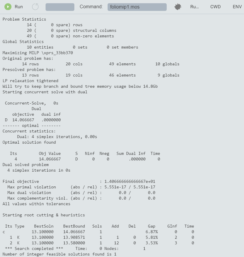
setparam("XPRS_VERBOSE",true)into the model before the call to maximize and re-run the model. There are now more rows (constraints) and columns (variables) than in the LP matrix of the previous chapters.

Figure 7.1: Solver log for MIP problem
As we have seen, it is relatively easy to turn an LP model into a MIP model by adding an integrality condition on some (or all) variables. However, the same does not hold for the solution algorithms: MIP problems are solved by repeatedly solving LP problems. Initially, the problem is solved without any integrality constraints (the LP relaxation). Then, one at a time, a discrete variable is chosen that does not satisfy the integrality condition in the current solution and new upper or lower bounds are added for this variable to bring it to an integer value. If we represent every LP solution as a node and connect these nodes by the bound changes or added constraints, then we obtain a tree-like structure, the Branch-and-Bound tree.
In particular, the branching information tells us how many Branch-and-Bound nodes have been needed to solve the problem: here it is just one, the enumeration did not even start. By default, Xpress Optimizer enables certain MIP pre-treatment algorithms (see the `Optimizer Reference Manual' for further detail on algorithmic settings), among others the automated generation of cuts—i.e., additional constraints that cut off parts of the LP solution space, but no solution of the MIP. This problem is of very small size and becomes so easy through the pre-treatment that it is solved immediately.
Add the lines
 setparam("XPRS_CUTSTRATEGY",0)
 setparam("XPRS_HEURSTRATEGY",0)
 setparam("XPRS_PRESOLVE",0)
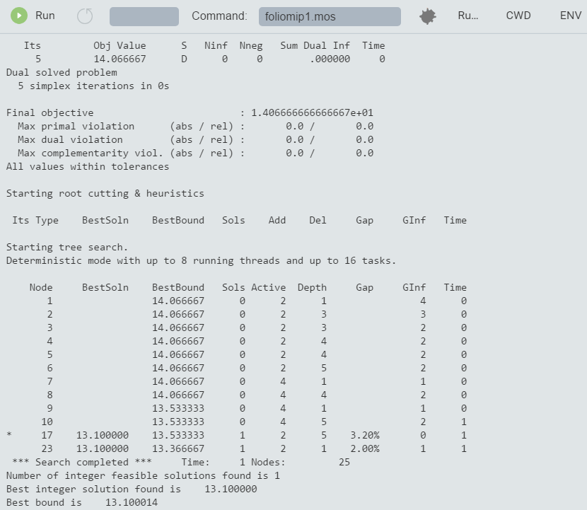
to your model before the call to maximize and re-execute it. You have now switched off the MIP pre-treatment routines for automated cut generation and MIP heuristics, and also the presolve mechanism (a treatment to the matrix that tries to reduce its size and improve its numerical properties).
It now takes several nodes to solve the problem:

Figure 7.2: Solver log for MIP problem with Branch-and-Bound
MIP model 2: imposing a minimum investment in each share
To formulate the second MIP model, we start again with the LP model from Chapters 2 and 3. The new constraint we wish to formulate is `if a share is bought, at least a certain minimum amount MINVAL = 10% of the budget is spent on the share.' Instead of simply constraining every variable fracs to take a value between 0 and MAXVAL, it now must either lie in the interval between MINVAL and MAXVAL or take the value 0. This type of variable is known as semi-continuous variable. In the new model, we replace the bounds on the variables fracs by the following constraint:
Implementation with Mosel
The following model foliomip2.mos implements the MIP model 2, again starting with the LP model from Chapter 3 augmented by the data initialization from file explained in Chapter 4. The semi-continuous variables are defined with the is_semcont constraint.
A similar type is available for integer variables that take either the value 0 or an integer value between a given limit and their upper bound (so-called semi-continuous integers): is_semint. A third composite type is a partial integer which takes integer values from its lower bound to a given limit value and is continuous beyond this value (marked by is_partint).
model "Portfolio optimization with MIP"
 uses "mmxprs"                      ! Use Xpress Optimizer

 parameters
  MAXRISK = 1/3                     ! Max. investment into high-risk values
  MINAM = 0.5                       ! Min. investment into N.-American values
  MAXVAL = 0.3                      ! Max. investment per share
  MINVAL = 0.1                      ! Min. investment per share
 end-parameters

 declarations
  SHARES: set of string             ! Set of shares
  RISK: set of string               ! Set of high-risk values among shares
  NA: set of string                 ! Set of shares issued in N.-America
  RET: array(SHARES) of real        ! Estimated return in investment
 end-declarations

 initializations from "folio.dat"
  RISK RET NA
 end-initializations

 declarations
  frac: array(SHARES) of mpvar      ! Fraction of capital used per share
 end-declarations

! Objective: total return
 Return:= sum(s in SHARES) RET(s)*frac(s)

! Limit the percentage of high-risk values
 sum(s in RISK) frac(s) <= MAXRISK

! Minimum amount of North-American values
 sum(s in NA) frac(s) >= MINAM

! Spend all the capital
 sum(s in SHARES) frac(s) = 1

! Upper and lower bounds on the investment per share
 forall(s in SHARES) do
  frac(s) <= MAXVAL
  frac(s) is_semcont MINVAL
 end-do

! Solve the problem
 maximize(Return)

! Solution printing
 writeln("Total return: ", getobjval)
 forall(s in SHARES) writeln(s, ": ", getsol(frac(s))*100, "%")

end-model
When executing this model of the solution information window) we obtain the following output:
Total return: 14.0333
treasury: 30%
hardware: 0%
theater: 20%
telecom: 0%
brewery: 10%
highways: 26.6667%
cars: 0%
bank: 0%
software: 13.3333%
electronics: 0%
Now five securities are chosen for the portfolio, each forming at least 10% and at most 30% of the total investment. Due to the additional constraint, the optimal MIP solution value is again lower than the initial LP solution value.

