Quadratic Programming
In this chapter we turn the LP problem from Chapter 3 into a Quadratic Programming (QP) problem, and the first MIP model from Chapter 6 into a Mixed Integer Quadratic Programming (MIQP) problem. The chapter shows how to
- define quadratic objective functions,
- incrementally define and solve problems,
- understand and exploit the MIP optimization displays.
Chapter 12 shows how to formulate and solve the same examples with BCL and in Chapter 17 the QP problem is input and solved directly with Xpress Optimizer.
Problem description
The investor may also look at his portfolio selection problem from a different angle: instead of maximizing the estimated return and limiting the portion of high-risk investments he now wishes to minimize the risk whilst obtaining a certain target yield. He adopts the Markowitz idea of getting estimates of the variance/covariance matrix of estimated returns on the securities. (For example, hardware and software company worths tend to move together, but are oppositely correlated with the success of theatrical production, as people go to the theater more when they have become bored with playing with their new computers and computer games.) The return on theatrical productions are highly variable, whereas the treasury bill yield is certain. The estimated returns and the variance/covariance matrix are given in the following table:
| treasury | hardw. | theater | telecom | brewery | highways | cars | bank | softw. | electr. | |
|---|---|---|---|---|---|---|---|---|---|---|
| treasury | 0.1 | 0 | 0 | 0 | 0 | 0 | 0 | 0 | 0 | 0 |
| hardware | 0 | 19 | -2 | 4 | 1 | 1 | 1 | 0.5 | 10 | 5 |
| theater | 0 | -2 | 28 | 1 | 2 | 1 | 1 | 0 | -2 | -1 |
| telecom | 0 | 4 | 1 | 22 | 0 | 1 | 2 | 0 | 3 | 4 |
| brewery | 0 | 1 | 2 | 0 | 4 | -1.5 | -2 | -1 | 1 | 1 |
| highways | 0 | 1 | 1 | 1 | -1.5 | 3.5 | 2 | 0.5 | 1 | 1.5 |
| cars | 0 | 1 | 1 | 2 | -2 | 2 | 5 | 0.5 | 1 | 2.5 |
| bank | 0 | 0.5 | 0 | 0 | -1 | 0.5 | 0.5 | 1 | 0.5 | 0.5 |
| software | 0 | 10 | -2 | 3 | 1 | 1 | 1 | 0.5 | 25 | 8 |
| electronics | 0 | 5 | -1 | 4 | 1 | 1.5 | 2.5 | 0.5 | 8 | 16 |
Question 1: Which investment strategy should the investor adopt to minimize the variance subject to getting some specified minimum target yield?
Question 2: Which is the least variance investment strategy if the investor wants to choose at most four different securities (again subject to getting some specified minimum target yield)?
The first question leads us to a Quadratic Programming problem, that is, a Mathematical Programming problem with a quadratic objective function and linear constraints. The second question necessitates the introduction of discrete variables to count the number of securities, and so we obtain a Mixed Integer Quadratic Programming problem. The two cases will be discussed separately in the following two sections.
QP
To adapt the model developed in Chapter 2 to the new way of looking at the problem, we need to make the following changes:
- New objective function: mean variance instead of total return.
- The risk-related constraint disappears.
- Addition of a new constraint: target yield.
The new objective function is the mean variance of the portfolio, namely:
where VARst is the variance/covariance matrix of all shares. This is a quadratic objective function (an objective function becomes quadratic either when a variable is squared, e.g., frac12, or when two variables are multiplied together, e.g., frac1 · frac2).
The target yield constraint can be written as follows:
The limit on the North-American shares as well as the requirement to spend all the money, and the upper bounds on the fraction invested into every share are retained. We therefore obtain the following complete mathematical model formulation:
∑s ∈ NA fracs ≥ MINAM
∑s ∈ SHARES fracs = 1
∑s ∈ SHARES RETs·fracs ≥ TARGET
∀ s ∈ SHARES: 0 ≤ fracs ≤ MAXVAL
Implementation with Mosel
In addition to the Xpress Optimizer module mmxprs we now also need to load the module mmnl that adds to the Mosel language the facilities required for the definition of quadratic expressions (mmnl is documented in the `Mosel Language Reference Manual'). We can then use the optimization function maximize (or alternatively minimize) for quadratic objective functions to start the solution process.
This model uses a different data file (folioqp.dat) than the previous models:
           ! trs  haw  thr  tel  brw  hgw  car  bnk  sof  elc
RET: [   (1)   5   17   26   12    8    9    7    6   31   21]

VAR: [ (1 1) 0.1    0    0    0    0    0    0    0    0    0 ! treasury
       (2 1)   0   19   -2    4    1    1    1  0.5   10    5 ! hardware
       (3 1)   0   -2   28    1    2    1    1    0   -2   -1 ! theater
       (4 1)   0    4    1   22    0    1    2    0    3    4 ! telecom
       (5 1)   0    1    2    0    4 -1.5   -2   -1    1    1 ! brewery
       (6 1)   0    1    1    1 -1.5  3.5    2  0.5    1  1.5 ! highways
       (7 1)   0    1    1    2   -2    2    5  0.5    1  2.5 ! cars
       (8 1)   0  0.5    0    0   -1  0.5  0.5    1  0.5  0.5 ! bank
       (9 1)   0   10   -2    3    1    1    1  0.5   25    8 ! software
      (10 1)   0    5   -1    4    1  1.5  2.5  0.5    8   16 ! electronics
     ]

RISK: [2 3 4 9 10]
NA: [1 2 3 4]
Note that we have chosen to use numerical instead of string indices. Since the set SHARES is defined in the model, we do not have to list the index-tuple for every data entry in the file—those tuples given are for clarity's sake only.
model "Portfolio optimization with QP/MIQP"
 uses "mmxprs", "mmnl"              ! Use Xpress Optimizer with QP solver

 parameters
  MAXVAL = 0.3                      ! Max. investment per share
  MINAM = 0.5                       ! Min. investment into N.-American values
  MAXNUM = 4                        ! Max. number of different assets
  TARGET = 9.0                      ! Minimum target yield
 end-parameters

 declarations
  SHARES = 1..10                    ! Set of shares
  RISK: set of integer              ! Set of high-risk values among shares
  NA: set of integer                ! Set of shares issued in N.-America
  RET: array(SHARES) of real        ! Estimated return in investment
  VAR: array(SHARES,SHARES) of real ! Variance/covariance matrix of
                                    ! estimated returns
 end-declarations

 initializations from "folioqp.dat"
  RISK RET NA VAR
 end-initializations

 declarations
  frac: array(SHARES) of mpvar      ! Fraction of capital used per share
 end-declarations

! Objective: mean variance
 Variance:= sum(s,t in SHARES) VAR(s,t)*frac(s)*frac(t)

! Minimum amount of North-American values
 sum(s in NA) frac(s) >= MINAM

! Spend all the capital
 sum(s in SHARES) frac(s) = 1

! Target yield
 sum(s in SHARES) RET(s)*frac(s) >=  TARGET

! Upper bounds on the investment per share
 forall(s in SHARES) frac(s) <= MAXVAL

! Solve the problem
 minimize(Variance)

! Solution printing
 writeln("With a target of ", TARGET, " minimum variance is ", getobjval)
 forall(s in SHARES) writeln(s, ": ", getsol(frac(s))*100, "%")

end-model
This model (file folioqp.mos) produces the following solution output (tab Output/input of the solution information window):
With a target of 9 minimum variance is 0.557393
1: 30%
2: 7.15391%
3: 7.38246%
4: 5.46363%
5: 12.6554%
6: 5.91228%
7: 0.332458%
8: 30%
9: 1.09983%
10: 0%
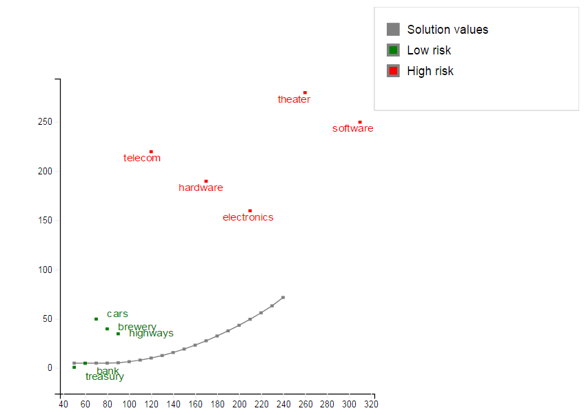
Similarly to the algorithm shown in Chapter 5, we may re-solve this problem with different values of TARGET and plot the results in a target return/standard deviation graph, know as the `efficient frontier' (model file folioqp_graph.mos):

Figure 8.1: Graph of the efficient frontier
MIQP
We now wish to express the fact that at most a given number MAXNUM of different assets may be selected into the portfolio, subject to all other constraints of the previous QP model. In Chapter 6 we have already seen how this can be done, namely by introducing an additional set of binary decision variables buys that are linked logically to the continuous variables:
Through this relation, a variable buys will be at 1 if a fraction fracs greater than 0 is selected into the portfolio. If, however, buys equals 0, then fracs must also be 0.
To limit the number of different shares in the portfolio, we then define the following constraint:
Implementation with Mosel
We may modify the previous QP model or simply add the following lines to the end of the QP model in the previous section: the problem is then solved once as a QP and once as a MIQP in a single model run.
 declarations
  buy: array(SHARES) of mpvar       ! 1 if asset is in portfolio, 0 otherwise
 end-declarations

! Limit the total number of assets
 sum(s in SHARES) buy(s) <= MAXNUM

 forall(s in SHARES) do
  buy(s) is_binary
  frac(s) <= buy(s)
 end-do

! Solve the problem
 minimize(Variance)

 writeln("With a target of ", TARGET," and at most ", MAXNUM,
         " assets, minimum variance is ", getobjval)
 forall(s in SHARES) writeln(s, ": ", getsol(frac(s))*100, "%")
When executing the MIQP model, we obtain the following solution output:
With a target of 9 and at most 4 assets,
 minimum variance is 1.24876
1: 30%
2: 20%
3: 0%
4: 0%
5: 23.8095%
6: 26.1905%
7: 0%
8: 0%
9: 0%
10: 0%
With the additional constraint on the number of different assets the minimum variance is more than twice as large as in the QP problem.
Analyzing the solution
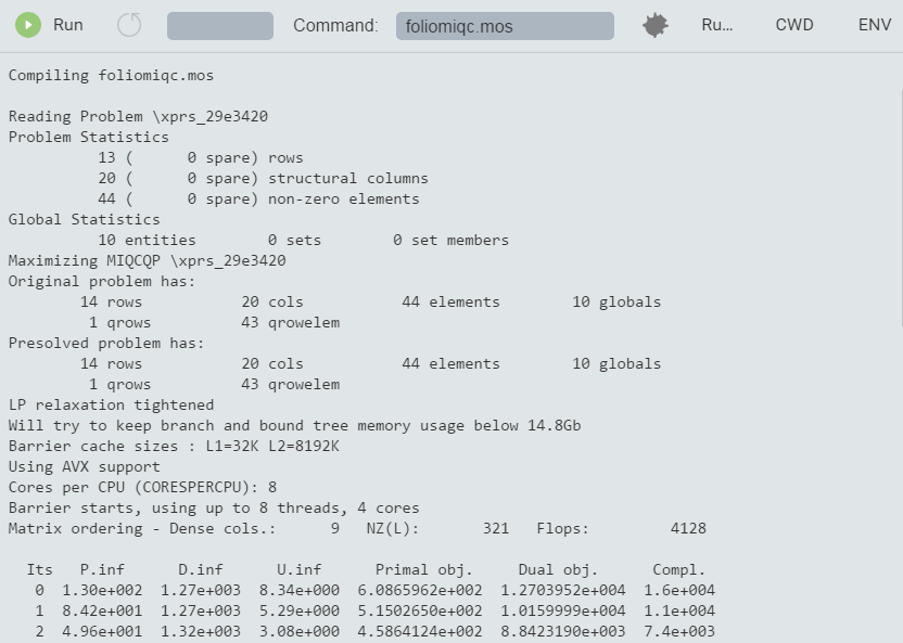
If we enable the Optimizer logging output display by setting XPRS_VERBOSE to 'true' we see the following information:

Figure 8.2: Detailed MIQP solution information
This is quite similar to the MIP statistics, perhaps with the exception of the LP solution algorithm: the initial LP relaxation has been solved by the Newton-Barrier algorithm.
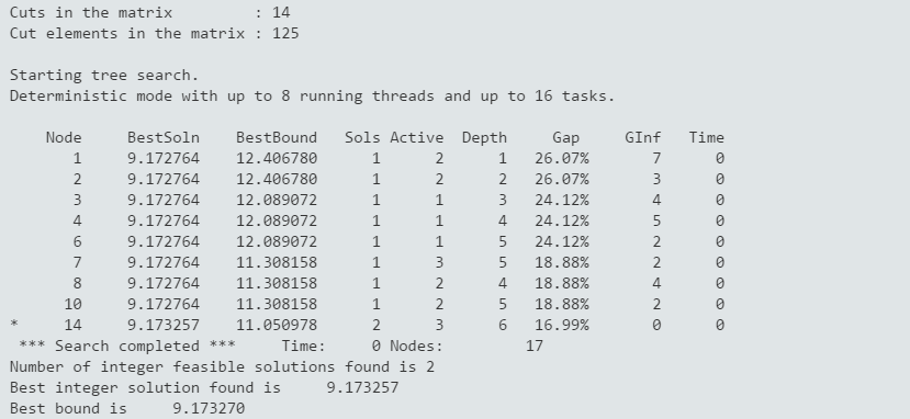
During the search, two integer feasible solutions have been found, the first during the root cutting and heuristics phase:

Figure 8.3: MIQP root cutting and heuristics
and the second during the Branch-and-Bound search. The search has been completed, this means that optimality of this solution has been proven (we may have chosen to stop the search, for example, after a given number of nodes, in which case it may not be possible to prove optimality or even to find the best solution).

Figure 8.4: MIQP Branch-and-Bound search

