
Non-linear functions
Can model non-linear functions in the same way as incremental pricebreaks
- approximate the non-linear function with a piecewise linear function
- use an SOS2 to model the piecewise linear function
Non-linear function in a single variable
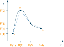
- x-coordinates of the points: R1, ..., R4
y-coordinates F1, ..., F4. So point 1 is (R1,F1) etc. - Let weights (decision variables) associated with point i be wi (i=1,...,4)
- Form convex combinations of the points using weights wi to get a combination point (x,y):
where the variables wi form an SOS2 set with ordering coefficients defined by values Ri.x = ∑i wi·Ri y = ∑i wi·Fi ∑i wi = 1 - Mosel implementation:
 declarations
  I=1..4
  x,y: mpvar
  w: array(I) of mpvar
  R,F: array(I) of real
 end-declarations

! ...assign values to arrays R and F...

! Define the SOS-2 with "reference row" coefficients from R
 Defx:= sum(i in I) R(i)*w(i) is_sos2
 sum(i in I) w(i) = 1

! The variable and the corresponding function value we want to approximate
 x = Defx
 y = sum(i in I) F(i)*w(i)
- BCL implementation:
 XPRBprob prob("testsos");
 XPRBvar x, y, w[I];
 XPRBexpr Defx, le, ly;
 double R[I], F[I];
 int i;

// ...assign values to arrays R and F...

// Create the decision variables
 x = prob.newVar("x"); y = prob.newVar("y");
 for(i=0; i<I; i++) w[i] = prob.newVar("w");

// Define the SOS-2 with "reference row" coefficients from R
 for(i=0; i<I; i++) Defx += R[i]*w[i];
 prob.newSos("Defx", XPRB_S2, Defx);
 for(i=0; i<I; i++) le += w[i];
 prob.newCtr("One", le == 1);

// The variable and the corresponding function value we want to approximate
 prob.newCtr("Eqx", x == Defx);
 for(i=0; i<I; i++) ly += F[i]*w[i];
 prob.newCtr("Eqy", y == ly);
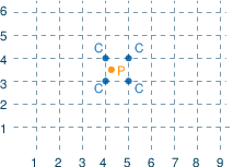
Non-linear function in two variables
Interpolation of a function f in two variables: approximate f at a point P by the corners C of the enclosing square of a rectangular grid (NB: the representation of P=(x,y) by the four points C obviously means a fair amount of degeneracy).
- x-coordinates of grid points: X1, ..., Xn
y-coordinates of grid points: Y1, ..., Ym. So grid points are (Xi,Yj). - Function evaluation at grid points: FXY11, ..., FXYnm
- Define weights (decision variables) associated with x and y coordinates, wxi respectively wyj, and for each grid point (X(i),Y(j)) define a variable wxyij
- Form convex combinations of the points using the weights to get a combination point (x,y) and the corresponding function approximation:
where the variables wxi form an SOS2 set with ordering coefficients defined by values Xi, and the variables wyj are a second SOS2 set with coordinate values Yj as ordering coefficients.x = ∑i wxi·Xi y = ∑j wyj·Yj f = ∑ij wxyij·FXYij ∀ i=1,...,n: ∑j wxyij = wxi ∀ j=1,...,m: ∑i wxyij = wyj ∑i wxi = 1 ∑j wyj = 1 - Mosel implementation:
 declarations
  RX,RY:range
  X: array(RX) of real          ! x coordinate values of grid points
  Y: array(RY) of real          ! y coordinate values of grid points
  FXY: array(RX,RY) of real     ! Function evaluation at grid points
 end-declarations

! ... initialize data

 declarations
  wx: array(RX) of mpvar        ! Weight on x coordinate
  wy: array(RY) of mpvar        ! Weight on y coordinate
  wxy: array(RX,RY) of mpvar    ! Weight on (x,y) coordinates
  x,y,f: mpvar
 end-declarations

! Definition of SOS (assuming coordinate values <>0)
 sum(i in RX) X(i)*wx(i) is_sos2
 sum(j in RY) Y(j)*wy(j) is_sos2

! Constraints
 forall(i in RX) sum(j in RY) wxy(i,j) = wx(i)
 forall(j in RY) sum(i in RX) wxy(i,j) = wy(j)
 sum(i in RX) wx(i) = 1
 sum(j in RY) wy(j) = 1

! Then x, y and f can be calculated using
 x = sum(i in RX)  X(i)*wx(i)
 y = sum(j in RY)  Y(j)*wy(j)
 f = sum(i in RX,j in RY) FXY(i,j)*wxy(i,j)

! f can take negative or positive values (unbounded variable)
 f is_free
 XPRBprob prob("testsos");
 XPRBvar x, y, f;
 XPRBvar wx[NX], wy[NY], wxy[NX][NY];       // Weights on coordinates
 XPRBexpr Defx, Defy, le, lexy, lx, ly;
 double DX[NX], DY[NY];
 double FXY[NX][NY];
 int i,j;

// ... initialize data arrays DX, DY, FXY

// Create the decision variables
 x = prob.newVar("x"); y = prob.newVar("y");
 f = prob.newVar("f", XPRB_PL, -XPRB_INFINITY, XPRB_INFINITY);   // Unbounded variable
 for(i=0; i<NX; i++) wx[i] = prob.newVar("wx");
 for(j=0; j<NY; j++) wy[j] = prob.newVar("wy");
 for(i=0; i<NX; i++)
  for(j=0; j<NY; j++) wxy[i][j] = prob.newVar("wxy");

// Definition of SOS
 for(i=0; i<NX; i++) Defx += X[i]*wx[i];
 prob.newSos("Defx", XPRB_S2, Defx);
 for(j=0; j<NY; j++) Defy += Y[j]*wy[j];
 prob.newSos("Defy", XPRB_S2, Defy);

// Constraints
 for(i=0; i<NX; i++) {
  le = 0;
  for(j=0; j<NY; j++) le += wxy[i][j];
  prob.newCtr("Sumx", le == wx[i]);
 }
 for(j=0; j<NY; j++) {
  le = 0;
  for(i=0; i<NX; i++) le += wxy[i][j];
  prob.newCtr("Sumy", le == wy[j]);
 }
 for(i=0; i<NX; i++) lx += wx[i];
 prob.newCtr("Convx", lx == 1);
 for(j=0; j<NY; j++) ly += wy[j];
 prob.newCtr("Convy", ly == 1);

// Calculate x, y and the corresponding function value f we want to approximate
 prob.newCtr("Eqx", x == Defx);
 prob.newCtr("Eqy", y == Defy);
 for(i=0; i<NX; i++)
  for(j=0; j<NY; j++) lexy += FXY[i][j]*wxy[i][j];
 prob.newCtr("Eqy", f == lexy);