Extensions: setup times, resource choice, usage profiles

Setup times

Consider once more the problem of planning the production of paint batches introduced in Section implies: Paint production. Between the processing of two batches the machine needs to be cleaned. The cleaning (or setup) times incurred are sequence-dependent and asymetric. The objective is to determine a production cycle of the shortest length.

Model formulation

For every job j (j ∈ JOBS = {1,...,NJ}), represented by a task object task_j, we are given its processing duration DUR_j. We also have a matrix of cleaning times CLEAN with entries CLEAN_jk indicating the duration of the cleaning operation if task k succedes task j. The machine processing the jobs is modeled as a resource res of unitary capacity, thus stating the disjunctions between the jobs.

With the objective to minimize the makespan (completion time of the last batch) we obtain the following model:

resource res
tasks task_j (j ∈ JOBS)
minimize finish
finish = maximum_{j ∈ JOBS}(task_j.end)
res.capacity = 1
∀ j ∈ JOBS: task_j.duration = DUR_j
∀ j ∈ JOBS: task_j.requirement_res = 1
∀ j,k ∈ JOBS: setup(task_j, task_k) = CLEAN_jk

The tricky bit in the formulation of the original problem is that we wish to minimize the cycle time, that is, the completion of the last job plus the setup required between the last and the first jobs in the sequence. Since our task-based model does not contain any information about the sequence or rank of the jobs we introduce auxiliary variables firstjob and lastjob for the index values of the jobs in the first and last positions of the production cycle, and a variable cleanlf for the duration of the setup operation between the last and first tasks. The following constraints express the relations between these variables and the task objects:

firstjob, lastjob ∈ JOBS
firstjob ≠ lastjob
∀ j ∈ JOBS: task_j.end = finish ⇒ lastjob = j
∀ j ∈ JOBS: task_j.start = 1 ⇒ firstjob = j
cleanlf = CLEAN_{lastjob,firstjob}

Minimizing the cycle time then corresponds to minimizing the sum finish + cleanlf.

Implementation

The following Mosel model implements the task-based model formulated above. The setup times between tasks are set with the procedure setsetuptimes indicating the two task objects and the corresponding duration value.

model "B-5 Paint production (CP)"
 uses "kalis"

 declarations
  NJ = 5                             ! Number of paint batches (=jobs)
  JOBS=1..NJ

  DUR: array(JOBS) of integer        ! Durations of jobs
  CLEAN: array(JOBS,JOBS) of integer ! Cleaning times between jobs

  task: array(JOBS) of cptask
  res: cpresource

  firstjob,lastjob,cleanlf,finish: cpvar
  L: cpvarlist
  cycleTime: cpvar                   ! Objective variable
  Strategy: array(range) of cpbranching
 end-declarations

 initializations from 'Data/b5paint.dat'
  DUR CLEAN
 end-initializations

! Setting up the resource (formulation of the disjunction of tasks)
 set_resource_attributes(res, KALIS_UNARY_RESOURCE, 1)

! Setting up the tasks
 forall(j in JOBS) getstart(task(j)) >= 1                     ! Start times
 forall(j in JOBS) set_task_attributes(task(j), DUR(j), res)  ! Dur.s + disj.
 forall(j,k in JOBS) setsetuptime(task(j), task(k), CLEAN(j,k), CLEAN(k,j))
                                     ! Cleaning times between batches

! Cleaning time at end of cycle (between last and first jobs)
 setdomain(firstjob, JOBS); setdomain(lastjob, JOBS)
 firstjob <> lastjob
 forall(j in JOBS) equiv(getend(task(j))=getmakespan, lastjob=j)
 forall(j in JOBS) equiv(getstart(task(j))=1, firstjob=j)
 cleanlf = element(CLEAN, lastjob, firstjob)

 forall(j in JOBS) L += getend(task(j))
 finish = maximum(L)

! Objective: minimize the duration of a production cycle
 cycleTime = finish - 1 + cleanlf

! Solve the problem
 if cp_schedule(cycleTime) = 0 then
  writeln("Problem is infeasible")
  exit(1)
 end-if
 cp_show_stats

! Solution printing
 declarations
  SUCC: array(JOBS) of integer
 end-declarations

 forall(j in JOBS)
  forall(k in JOBS)
   if getsol(getstart(task(k))) = getsol(getend(task(j)))+CLEAN(j,k) then
    SUCC(j):= k
    break
   end-if
 writeln("Minimum cycle time: ", getsol(cycleTime))
 writeln("Sequence of batches:\nBatch Start Duration Cleaning")
 forall(k in JOBS)
  writeln("  ", k, strfmt(getsol(getstart(task(k))),7), strfmt(DUR((k)),8),
          strfmt(if(SUCC(k)>0, CLEAN(k,SUCC(k)), getsol(cleanlf)),9))

end-model

Results

The results are similar to those reported in Section implies: Paint production. It should be noted here that this model formulation is less efficient, in terms of search nodes and running times, than the previous model versions, and in particular the 'cycle' constraint version presented in Section cycle: Paint production. However, the task-based formulation is more generic and easier to extend with additional features than the problem-specific formulations in the previous model versions.

The graphical representation of the results looks as follows (Figure Solution graph).

Figure 5.4: Solution graph

Alternative resources

Quite frequently in scheduling applications the assignment of tasks to resources is not entirely fixed from the outset. For instance, there may be a group of resources (identical or not) among which to choose for a given processing step. If the resources are identical the task will have the same properties (duration, amount of resource use/provision/consumption/production) independent of the resource used for its processing. Otherwise, if resources are non-identical there is some resource-dependent data component.

We shall show here how to formulate a tiny example of four tasks that may be processed by two non-identical machines. Each task must be assigned to a single machine. The resource usage per task depends on the machine it is assigned to.

Model formulation

For each task j in the set of tasks TASKS we are given a fixed duration DUR_j and a machine-dependent amount of resource REQ_jm that is required per time unit for the whole duration of the task. Both machines have the same capacity CAP.

The resulting model looks as follows.

resource res_m (m ∈ MACH)
tasks task_j (j ∈ TASKS)
minimize makespan
∀ m ∈ MACH: res_m.capacity = CAP
∀ j ∈ TASKS: task_j.start,task_j.end ∈ {0,...,HORIZON}
∀ j ∈ TASKS: task_j.duration = DUR_t
∀ j ∈ TASKS,m ∈ MACH: task_j.assignment_resm ∈ {0,1}
∀ j ∈ TASKS:

∑

m ∈ MACH

task_j.assignment_resm = 1
∀ j ∈ TASKS,m ∈ MACH: task_j.requirement_resm ∈ {0,REQ_jm}

Implementation

This is a Mosel implementation of the scheduling problem with alternative resources.

 uses "kalis"

 setparam("KALIS_DEFAULT_LB", 0)

 declarations
  TASKS = {"a","b","c","d"}           ! Index set of tasks
  MACH = {"M1", "M2"}                 ! Index set of resources
  USE: array(TASKS,MACH) of integer   ! Machine-dependent res. requirement
  DUR: array(TASKS) of integer        ! Durations of tasks

  T: array(TASKS) of cptask           ! Tasks
  R: array(MACH) of cpresource        ! Resources
 end-declarations

 DUR::(["a","b","c","d"])[7, 9, 8, 5]
 USE::(["a","b","c","d"],["M1","M2"])[
      4, 3,
      2, 3,
      2, 1,
      4, 5]

! Define discrete resources
 forall(m in MACH)
  set_resource_attributes(R(m), KALIS_DISCRETE_RESOURCE, 5)

! Define tasks with machine-dependent resource usages
 forall(j in TASKS) do
  T(j).duration:= DUR(j)
  T(j).name:= j
  requires(T(j), union(m in MACH) {resusage(R(m), USE(j,m))})
 end-do

 cp_set_solution_callback("print_solution")
 starttime:=timestamp

! Solve the problem
 if cp_schedule(getmakespan)=0 then
  writeln("No solution")
  exit(0)
 end-if

! Solution printing
 forall(j in TASKS)
  writeln(j, ": ", getsol(getstart(T(j))), " - ", getsol(getend(T(j))))
 forall(t in 1..getsol(getmakespan)) do
  write(strfmt(t-1,2), ": ")

  ! We cannot use 'getrequirement' here to access solution information
  ! (it returns a value corresponding to the current state, that is 0)
  forall(j in TASKS | t>getsol(getstart(T(j))) and t<=getsol(getend(T(j))))
   write(j, ":",
         sum(m in MACH) USE(j,m)*getsol(getassignment(T(j),R(m))), "  " )
  writeln
 end-do

! ****************************************************************

! Print solutions during enumeration at the node where they are found
 procedure print_solution
  writeln(timestamp-starttime, "sec. Solution: ", getsol(getmakespan))

  forall(m in MACH) do
   writeln(m, ":")

   forall(t in 0..getsol(getmakespan)-1) do
    write(strfmt(t,2), ": ")
    forall(j in TASKS | getrequirement(T(j), R(m), t)>0)
     write(j, ":", getrequirement(T(j), R(m), t), "  " )
    writeln(" (total ", sum(j in TASKS) getrequirement(T(j), R(m), t), ")" )
   end-do

  end-do
 end-procedure

end-model

A new feature introduced by this example are the resusage objects that are employed in the definition of the resource requirement constraints for the tasks. A resusage consists of a resource object and a resource usage (specified by a constant, lower and upper bounds, or a complete profile — see Section Resource profiles). In this example we use the simplest version with a fixed resource usage value. Optional third and forth arguments to requires can be defined to specify the minimum and maximum number of resources to be used by a task. The default version (employed in this example) will choose a single resource from the set of alternative resources.

The implementation also shows how to retrieve solution information about resource assignments at a solution node (that is, during the enumeration) and after the search. At the solution node the function getrequirement returns the desired resource usage information; for a solution summary after terminating the search we need to work with the decision variable obtained through getassignment.

The formulation of produces, consumes, and provides constraints with resusage objects is analogous to what we have shown here for requires.

Note: when implementing alternative resources you always have to use the resource type KALIS_DISCRETE_RESOURCES, setting a capacity limit of 1 for modeling disjunctive resources.

Results

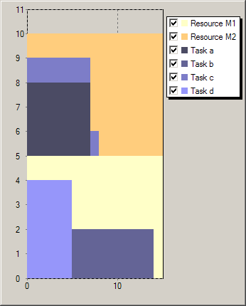
Figure Solutions for scheduling with resource choice shows two solutions generated by the execution of our model. The first solution uses a lesser total amount resource but the second one is optimal with respect to the objective of minimizing the makespan.

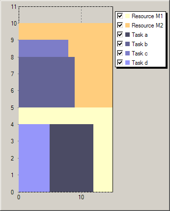Figure 5.5: Solutions for scheduling with resource choice

Note: leaving the decision about the resource choice open for the solver considerably increases the complexity of a scheduling problem. We therefore recommend to use this feature sparingly. Optimization problems involving resource assignment and sequencing aspects are often more easily solved by a decompostion approach (see the Xpress Whitepaper Hybrid MIP/CP solving with Xpress Optimizer and Xpress Kalis).

Resource profiles

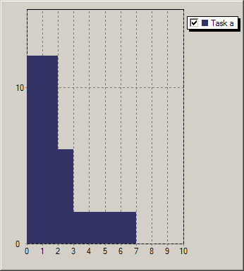
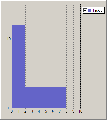
In all preceding examples we have worked with the assumption that a task is defined by a constant, though not necessarily fixed resource requirement (respectively resource provision, consumption, or production). Following this line of thought, a sequence of processesing steps with different resource usages would be represented by a corresponding number of tasks, each with a constant resource usage. However, the number of cptask objects required by such a formulation may be prohibitively large. Kalis therefore offers the possibility to define profiled tasks, that is, tasks with a non-constant resource usage profile. A task resource usage profile states for every time unit of the execution of the task the corresponding amount of resource. For example the four tasks in Figure Task profiles have the profiles Profile_a: (12, 12, 6, 2, 2, 2, 2), Profile_b: (12, 12, 6, 2, 2, 2, 2, 2, 2), Profile_c: (12, 12, 3, 3, 3, 3, 3, 3), and Profile_d: (6, 6, 6, 6, 6) respectively.

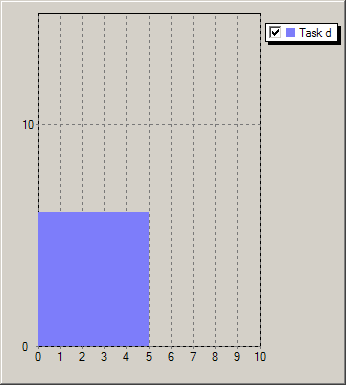Figure 5.6: Task profiles

Model formulation

Let TASKS = {'a','b','c','d'} be the set of tasks and res a resource of capacity CAP required by all tasks for their execution. With the objective of minimizing the makespan of the schedule we may formulate the model as follows.

resource res
tasks task_j (j ∈ TASKS)
minimize makespan
res.capacity = CAP
∀ j ∈ TASKS: task_j.start,task_j.end ∈ {0,...,HORIZON}
∀ j ∈ TASKS: task_j.duration = DUR_j
∀ j ∈ TASKS: task_j.requirement_res = Profile_j

This model formulation differs from a standard cumulative scheduling model (see Section Cumulative scheduling: discrete resources only in a single point: the resource requirement Profile_j of a task j is a list of values and not just a single constant.

Implementation

Let us now take a look at the model formulation with Mosel.

 uses "kalis"

 setparam("KALIS_DEFAULT_LB", 0)

 declarations
  TASKS = {"a","b","c","d"}           ! Index set of tasks
  Profile: array(TASKS) of list of integer   ! Task profiles
  DUR: array(TASKS) of integer        ! Durations of tasks

  T: array(TASKS) of cptask           ! Tasks
  R: cpresource                       ! Cumulative resource
 end-declarations

 DUR::(["a","b","c","d"])[7, 9, 8, 5]
 Profile("a"):= [12, 12, 6, 2, 2, 2, 2]
 Profile("b"):= [12, 12, 6, 2, 2, 2, 2, 2, 2]
 Profile("c"):= [12, 12, 3, 3, 3, 3, 3, 3]
 Profile("d"):= [6, 6, 6, 6, 6]

! Define a discrete resource
 set_resource_attributes(R, KALIS_DISCRETE_RESOURCE, 18)
 R.name:="machine"

! Define tasks with profiled resource usage
 forall(t in TASKS) do
  T(t).duration:= DUR(t)
  T(t).name:= t
  requires(T(t), resusage(R, Profile(t)))
 end-do

 cp_set_solution_callback("print_solution")
 starttime:=timestamp

! Solve the problem
 if cp_schedule(getmakespan)=0 then
  writeln("No solution")
  exit(0)
 end-if

! Solution printing
 writeln("Schedule with makespan ", getsol(getmakespan), ":")
 forall(t in TASKS)
  writeln(t, ": ", getsol(getstart(T(t))), " - ", getsol(getend(T(t))))

! ****************************************************************

! Print solutions during enumeration at the node where they are found.
! 'getrequirement' can only be used here to access solution information,
! not after the enumeration (it returns a value corresponding to the
! current state, that is, 0 after the enumeration).
 procedure print_solution
  writeln(timestamp-starttime, "sec. Solution: ", getsol(getmakespan))

  forall(i in 0..getsol(getmakespan)-1) do
   write(strfmt(i,2), ": ")
   forall(t in TASKS | getrequirement(T(t), R, i)>0)
    write(t, ":", getrequirement(T(t), R, i), "  " )
   writeln(" (total ", sum(t in TASKS) getrequirement(T(t), R, i), ")" )
  end-do
 end-procedure

end-model

The statement of the resource constraints (requires) uses an additional type of scheduling object for the definition of the resource profiles, namely resusage. We have already encountered this object in Section Alternative resources where it was employed in the definition of sets of alternative resources. In the present case there is only a single resource that must be used by all tasks, we now employ resusage to define resource usage profiles.

Results

The chart in Figure Solution for scheduling with resource profile shows an optimal schedule of the four tasks on a resource with capacity 18. All tasks are completed by time 11.

Figure 5.7: Solution for scheduling with resource profile

Resource idle times and preemption of tasks

In the examples of cumulative scheduling we have looked at so far resources are defined with a fixed constant capacity. In reality, it often happens that the resource availability is not constant over time: a resource 'staff', for instance, is likely to show variations corresponding to the presence or absence of personnel. Such changes to the resource level can be defined periodwise with the subroutine setcapacity. In the case of machine resources there may be scheduled downtimes for maintenance or other breaks, such as week-ends, relating to working hours. Any such periods that are known from the outset should be marked as 'unavailable for processing tasks'.

From the perspective of tasks there are two cases of resource unavailability: (1) any task starting before the resource unavailability must also be finished before the begin of this period (generally known as non-preemptive scheduling), and (2) a task started before the unavailability resumes its processing once the resource becomes available again (the case of preemptive scheduling).

With Kalis, the first case applies when resource capacities are set to 0 using setcapacity (independent of the type of the task). The second case is modeled by using profiled tasks and indicating resource unavailability with setidletimes.

For simplicity's sake, we merely consider two tasks, a and b, that are to be scheduled on a resource of capacity 3 that is unavailable in certain time periods. Task a has a constant resource requirement of 1 for 4 units of time, task b has the resource usage profile (1,1,1,2,2,2,1,1). Both tasks are preemptive.

Model formulation

Let TASKS = {'a','b'} be the set of tasks and res a resource of capacity CAP required by the tasks for their execution. The set IDLESET contains the time periods during which the resource is unavailable preempting the processing of tasks. With the objective of minimizing the makespan of the schedule we may formulate the model as follows.

resource res
tasks task_j (j ∈ TASKS)
minimize makespan
res.capacity = CAP
res.idletimes = IDLESET
∀ j ∈ TASKS: task_j.start,task_j.end ∈ {0,...,HORIZON}
∀ j ∈ TASKS: task_j.duration ≥ DUR_j
∀ j ∈ TASKS: task_j.requirement_res = Profile_j

Please notice that we do not fix the durations of the tasks in this formulation: we may indicate (lower or upper) bounds to restrict the total duration of a task, but if we want to leave room for preemptions the bounds on the durations of tasks must include some slack.

Implementation

The following model shows how to implement our example problem with Mosel.

model "Preemption"
 uses "kalis"

 setparam("KALIS_DEFAULT_LB", 0)

 declarations
  aprofile,bprofile: list of integer
  a,b: cptask
  R: cpresource
 end-declarations

! Define a discrete resource
 set_resource_attributes(R, KALIS_DISCRETE_RESOURCE, 3)

! Create a 'hole' in the availability of the resource:
! Uncomment one of the following two lines to compare their effect
! setcapacity(R, 1, 2, 0);  setcapacity(R, 7, 8, 0)
 setidletimes(R, (1..2)+(7..8))

! Define two tasks (a: constant resource use, b: resource profile)
 a.duration >= 4
 a.name:= "task_a"
 aprofile:= [1,1,1,1]

 b.duration >= 8
 b.name:= "task_b"
 bprofile:= [1,1,1,2,2,2,1,1]

! Resource usage constraints
 requires(a, resusage(R,aprofile))
 requires(b, resusage(R,bprofile))

 cp_set_solution_callback("print_solution")

! Solve the problem
 if cp_schedule(getmakespan)<>0 then
  cp_show_sol
 else
  writeln("No solution")
 end-if

! ****************************************************************

 procedure print_solution
  writeln("Solution: ", getsol(getmakespan))
  writeln("Schedule: a: ", getsol(getstart(a)), "-", getsol(getend(a))-1,
          ", b: ", getsol(getstart(b)), "-", getsol(getend(b))-1)
  writeln("Resource usage:")
  forall(t in 0..getsol(getmakespan)-1)
   writeln(strfmt(t,5), ": Cap: ", getcapacity(R,t), ", a:",
           getrequirement(a, R, t), ", b:", getrequirement(b, R, t))
 end-procedure

end-model

There are several equivalent ways of stating the constant resource usage of task a. Instead of defining explicitly the complete profile we may simply write

 requires(a, resusage(R,1)) 

or even shorter:

 requires(a, 1, R) 

Results

The model shown above produces the following solution output.

Solution: 12
Schedule: a: 0-5, b: 0-11
Resource usage:
    0: Cap: 3, a:1, b:1
    1: Cap: 3, a:0, b:0
    2: Cap: 3, a:0, b:0
    3: Cap: 3, a:1, b:1
    4: Cap: 3, a:1, b:1
    5: Cap: 3, a:1, b:2
    6: Cap: 3, a:0, b:2
    7: Cap: 3, a:0, b:0
    8: Cap: 3, a:0, b:0
    9: Cap: 3, a:0, b:2
   10: Cap: 3, a:0, b:1
   11: Cap: 3, a:0, b:1

The same model, replacing the line

 setidletimes(R, (1..2)+(7..8)) 

by this version indicating non-preemptive resource unavailability

 setcapacity(R, 1, 2, 0);  setcapacity(R, 7, 8, 0) 

results in the following solution where the tasks are placed in such a way that they do not overlap with any 'hole' in resource availability.

Solution: 17
Schedule: a: 3-6, b: 9-16
Resource usage:
    0: Cap: 3, a:0, b:0
    1: Cap: 0, a:0, b:0
    2: Cap: 0, a:0, b:0
    3: Cap: 3, a:1, b:0
    4: Cap: 3, a:1, b:0
    5: Cap: 3, a:1, b:0
    6: Cap: 3, a:1, b:0
    7: Cap: 0, a:0, b:0
    8: Cap: 0, a:0, b:0
    9: Cap: 3, a:0, b:1
   10: Cap: 3, a:0, b:1
   11: Cap: 3, a:0, b:1
   12: Cap: 3, a:0, b:2
   13: Cap: 3, a:0, b:2
   14: Cap: 3, a:0, b:2
   15: Cap: 3, a:0, b:1
   16: Cap: 3, a:0, b:1
 

It is also possible to define both, preemptive and non-preemptive times of unavailability for the same resource. For example, if times 1-2 correspond to a weekend where products may remain on the machine R and times 7-8 are required for maintenance operations during which the machine must imperatively be empty we would state in our model:

 setidletimes(R, 1, 2, 0)
 setcapacity(R, (7..8)) 

In this case the execution of task a may start at time 0, whereas task b will again be processed in times 9-16.