Renewable and non-renewable resources
Besides the distinction `disjunctive–cumulative' or `unary–discrete' that we have encountered in the previous sections there are other ways of describing or classifying resources. Another important property is the concept of renewable versus non-renewable resources. The previous examples have shown instances of renewable resources (machine capacity, manpower etc.): the amount of resource used by a task is released at its completion and becomes available for other tasks. In the case of non-renewable resources (e.g. money, raw material, intermediate products), the tasks using the resource consume it, that is, the available quantity of the resource is diminuished by the amount used up by processing a task.
Instead of using resources tasks may also produce certain quantities of resource. Again, we may have tasks that provide an amount of resource during their execution (renewable resources) or tasks that add the result of their production to a stock of resource (non-renewable resources).
Let us now see how to formulate the following problem: we wish to schedule five jobs P1 to P5 representing two stages of a production process. P1 and P2 produce an intermediate product that is needed by the jobs of the final stage (P3 to P5). For every job we are given its minimum and maximum duration, its cost or, for the jobs of the final stage, its profit contribution. There may be two cases, namely model A: the jobs of the first stage produce a given quantity of intermediate product (such as electricity, heat, steam) at every point of time during their execution, this intermediate product is consumed immediately by the jobs of the final stage. Model B: the intermediate product results as ouput from the jobs of the first stage and is required as input to start the jobs of the final stage. The intermediate product in model A is a renewable resource and in model B we have the case of a non-renewable resource.
Model formulation
Let FIRST = {P1,P2} be the set of jobs in the first stage, FINAL = {P3,P4,P5} the jobs of the second stage, and the set JOBS the union of all jobs. For every job j we are given its minimum and maximum duration MINDj and MAXDj respectively. RESAMTj is the amount of resource needed as input or resulting as output from a job. Furthermore we have a cost COSTj for jobs j of the first stage and a profit PROFITj for jobs j of the final stage.
Model A (renewable resource)
The case of a renewable resource is formulated by the following model. Notice that the resource capacity is set to 0 indicating that the only available quantities of resource are those produced by the jobs of the first production stage.
tasks taskj (j ∈ JOBS)
maximize
| ∑ |
| j ∈ JOBS |
res.capacity = 0
∀ j ∈ JOBS: taskj.start,taskj.end ∈ {0,...,HORIZON}
∀ j ∈ JOBS: taskj.duration ∈ {MINDj,...,MAXDj}
∀ j ∈ FIRST: taskj.provisionres = RESAMTj
∀ j ∈ FINAL: taskj.requirementres = RESAMTj
Model B (non-renewable resource)
In analogy to the model A we formulate the second case as follows.
tasks taskj (j ∈ JOBS)
maximize
| ∑ |
| j ∈ JOBS |
res.capacity = 0
∀ j ∈ JOBS: taskj.start,taskj.end ∈ {0,...,HORIZON}
∀ j ∈ JOBS: taskj.duration ∈ {MINDj,...,MAXDj}
∀ j ∈ FIRST: taskj.productionres = RESAMTj
∀ j ∈ FINAL: taskj.consumptionres = RESAMTj
However, this model does not entirely correspond to the problem description above since the production of the intermediate product occurs at the start of a task. To remedy this problem we may introduce an auxiliary task Endj for every job j in the first stage. The auxiliary job has duration 0, the same completion time as the original job and produces the intermediate product in the place of the original job.
∀ j ∈ FIRST: taskEndj.duration = 0
∀ j ∈ FIRST: taskj.productionres = 0
∀ j ∈ FIRST: taskEndj.productionres = RESAMTj
Implementation
The following Mosel model implements case A. We use the default scheduling solver (function cp_schedule) indicating by the value true for the optional second argument that we wish to maximize the objective function.
model "Renewable resource"
 uses "kalis", "mmsystem"

 forward public procedure solution_found

 declarations
  FIRST = {'P1','P2'}
  FINAL = {'P3','P4','P5'}
  JOBS = FIRST+FINAL

  MIND,MAXD: array(JOBS) of integer  ! Limits on job durations
  RESAMT: array(JOBS) of integer  ! Resource use/production
  HORIZON: integer                ! Time horizon
  PROFIT: array(FINAL) of real    ! Profit from production
  COST: array(JOBS) of real       ! Cost of production
  CAP: integer                    ! Available resource quantity

  totalProfit: cpfloatvar
  task: array(JOBS) of cptask     ! Task objects for jobs
  intermProd: cpresource          ! Non-renewable resource (intermediate prod.)
 end-declarations

 initializations from 'Data/renewa.dat'
  [MIND,MAXD] as 'DUR' RESAMT HORIZON PROFIT COST CAP
 end-initializations

! Setting up resources
 set_resource_attributes(intermProd, KALIS_DISCRETE_RESOURCE, CAP)
 setname(intermProd, "IntP")

! Setting up the tasks
 forall(j in JOBS) do
  setname(task(j), j)
  setduration(task(j), MIND(j), MAXD(j))
  setdomain(getend(task(j)), 0, HORIZON)
 end-do

! Providing tasks
 forall(j in FIRST) provides(task(j), RESAMT(j), intermProd)

! Requiring tasks
 forall(j in FINAL) requires(task(j), RESAMT(j), intermProd)

! Objective function: total profit
 totalProfit = sum(j in FINAL) PROFIT(j)*getduration(task(j)) -
               sum(j in JOBS) COST(j)*getduration(task(j))
 cp_set_solution_callback("solution_found")
 setparam("KALIS_MAX_COMPUTATION_TIME", 30)

! Solve the problem
 starttime:= gettime
 if cp_schedule(totalProfit,true)=0 then
  exit(1)
 end-if

! Solution printing
 writeln("Total profit: ", getsol(totalProfit))
 writeln("Job\tStart\tEnd\tDuration")
 forall(j in JOBS)
  writeln(j, "\t ", getsol(getstart(task(j))), "\t ", getsol(getend(task(j))),
          "\t ", getsol(getduration(task(j))))

 public procedure solution_found
  writeln(gettime-starttime , " sec. Solution found with total profit = ",
          getsol(totalProfit))
  forall(j in JOBS)
   write(j, ": ", getsol(getstart(task(j))), "-", getsol(getend(task(j))),
          "(", getsol(getduration(task(j))), "), ")
  writeln
 end-procedure

end-model
The model for case B adds the two auxiliary tasks (forming the set ENDFIRST) that mark the completion of the jobs in the first stage. The only other difference are the task properties produces and consumes that define the resource constraints. We only repeat the relevant part of the model:
 declarations
  FIRST = {'P1','P2'}
  ENDFIRST = {'EndP1', 'EndP2'}
  FINAL = {'P3','P4','P5'}
  JOBS = FIRST+ENDFIRST+FINAL

  MIND,MAXD: array(JOBS) of integer  ! Limits on job durations
  RESAMT: array(JOBS) of integer  ! Resource use/production
  HORIZON: integer                ! Time horizon
  PROFIT: array(FINAL) of real    ! Profit from production
  COST: array(JOBS) of real       ! Cost of production
  CAP: integer                    ! Available resource quantity

  totalProfit: cpfloatvar
  task: array(JOBS) of cptask     ! Task objects for jobs
  intermProd: cpresource          ! Non-renewable resource (intermediate prod.)
 end-declarations

 initializations from 'Data/renewb.dat'
  [MIND,MAXD] as 'DUR' RESAMT HORIZON PROFIT COST CAP
 end-initializations

! Setting up resources
 set_resource_attributes(intermProd, KALIS_DISCRETE_RESOURCE, CAP)
 setname(intermProd, "IntP")

! Setting up the tasks
 forall(j in JOBS) do
  setname(task(j), j)
  setduration(task(j), MIND(j), MAXD(j))
  setdomain(getend(task(j)), 0, HORIZON)
 end-do

! Production tasks
 forall(j in ENDFIRST) produces(task(j), RESAMT(j), intermProd)
 forall(j in FIRST) getend(task(j)) = getend(task("End"+j))

! Consumer tasks
 forall(j in FINAL) consumes(task(j), RESAMT(j), intermProd)
Results
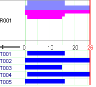
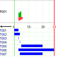
The behavior of the (default) search and the results of the two models are considerably different. The optimal solution with an objective of 344.9 for case B represented in Figure Solution for case B (resource production and consumption) is proven within a fraction of a second. Finding a good solution for case A takes several seconds on a standard PC; finding the optimal solution (see Figure Solution for case A (resource provision and requirement)) and proving its optimality requires several minutes of running time. The main reason for this poor behavior of the search is our choice of the objective function: the cost-based objective function does not propagate well and therefore does not help with pruning the search tree. A better choice for objective functions in scheduling problems generally are criteria involving the task decision variables (start, duration, or completion time, particularly the latter).

Figure 5.2: Solution for case A (resource provision and requirement)

Figure 5.3: Solution for case B (resource production and consumption)
Alternative formulation without scheduling objects
Instead of defining task and resource objects we may equally formulate this problem with a `producer-consumer' constraint over standard finite domain variables that represent the different attributes of tasks without being grouped into a predefined object. A single `producer-consumer' constraint expresses the problem of scheduling a set of tasks producing or consuming a non-renewable resource by establishing the following relations between its arguments (seven arrays of decision variables for the properties related to tasks—start, duration, end, per unit and cumulated resource production, per unit and cumulated resource consumption— all indexed by the same set R):
∀ j ∈ R: producej · durationj = psizej
∀ j ∈ R: consumej · durationj = csizej
∀ t ∈ TIMES:
| ∑ |
| j ∈ R | t ∈ [UB(startj)..LB(endj)] |
where UB stands for `upper bound' and LB for `lower bound' of a decision variable.
Implementation
The following Mosel model implements the second model version using the producer_consumer constraint.
model "Non-renewable resource"
 uses "kalis"

 setparam("KALIS_DEFAULT_LB", 0)

 declarations
  FIRST = {'P1','P2'}
  ENDFIRST = {'EndP1', 'EndP2'}
  FINAL = {'P3','P4','P5'}
  JOBS = FIRST+ENDFIRST+FINAL
  PCJOBS = ENDFIRST+FINAL

  MIND,MAXD: array(JOBS) of integer  ! Limits on job durations
  RESAMT: array(JOBS) of integer  ! Resource use/production
  HORIZON: integer                ! Time horizon
  PROFIT: array(FINAL) of real    ! Profit from production
  COST: array(JOBS) of real       ! Cost of production
  CAP: integer                    ! Available resource quantity

  totalProfit: cpfloatvar
  fstart,fdur,fcomp: array(FIRST) of cpvar! Start, duration & completion of jobs
  start,dur,comp: array(PCJOBS) of cpvar  ! Start, duration & completion of jobs
  produce,consume: array(PCJOBS) of cpvar ! Production/consumption per time unit
  psize,csize: array(PCJOBS) of cpvar     ! Cumulated production/consumption
 end-declarations

 initializations from 'Data/renewb.dat'
  [MIND,MAXD] as 'DUR' RESAMT HORIZON PROFIT COST CAP
 end-initializations

! Setting up the tasks
 forall(j in PCJOBS) do
  setname(start(j), j)
  setdomain(dur(j), MIND(j), MAXD(j))
  setdomain(comp(j), 0, HORIZON)
  start(j) + dur(j) = comp(j)
 end-do
 forall(j in FIRST) do
  setname(fstart(j), j)
  setdomain(fdur(j), MIND(j), MAXD(j))
  setdomain(fcomp(j), 0, HORIZON)
  fstart(j) + fdur(j) = fcomp(j)
 end-do

! Production tasks
 forall(j in ENDFIRST) do
  produce(j) = RESAMT(j)
  consume(j) = 0
 end-do
 forall(j in FIRST) fcomp(j) = comp("End"+j)

! Consumer tasks
 forall(j in FINAL) do
  consume(j) = RESAMT(j)
  produce(j) = 0
 end-do

! Resource constraint
 producer_consumer(start, comp, dur, produce, psize, consume, csize)

! Objective function: total profit
 totalProfit = sum(j in FINAL) PROFIT(j)*dur(j) -
               sum(j in FIRST) COST(j)*fdur(j)

 if not cp_maximize(totalProfit) then
  exit(1)
 end-if

 writeln("Total profit: ", getsol(totalProfit))
 writeln("Job\tStart\tEnd\tDuration")
 forall(j in FIRST)
  writeln(j, "\t ", getsol(fstart(j)), "\t ", getsol(fcomp(j)),
          "\t ", getsol(fdur(j)))
 forall(j in PCJOBS)
  writeln(j, "\t ", getsol(start(j)), "\t ", getsol(comp(j)),
          "\t ", getsol(dur(j)))

end-model
This model generates the same solution as the previous model version with a slightly longer running time (though still just a fraction of a second on a standard PC).
© 2001-2020 Fair Isaac Corporation. All rights reserved. This documentation is the property of Fair Isaac Corporation (“FICO”). Receipt or possession of this documentation does not convey rights to disclose, reproduce, make derivative works, use, or allow others to use it except solely for internal evaluation purposes to determine whether to purchase a license to the software described in this documentation, or as otherwise set forth in a written software license agreement between you and FICO (or a FICO affiliate). Use of this documentation and the software described in it must conform strictly to the foregoing permitted uses, and no other use is permitted.

