
Quadratically Constrained Quadratic Programs (QCQPs)
Quadratically Constrained Quadratic Programs (QCQPs) are an extension of the Quadratic Programming (QP) problem where the constraints may also include second order polynomials.
A QCQP problem may be written as:
| minimize: | c1x1+...+cnxn+xTQ0x | ||
| subject to: | a11x1+...+a1nxn+xTQ1x | ≤ | b1 |
| ... | |||
| am1x1+...+amnxn+xTQmx | ≤ | bm | |
| l1≤x1≤u1,...,ln≤xn≤un |
where any of the lower or upper bounds li or ui may be infinite.
The FICO Xpress Optimizer can be used directly for solving QCQP problems with support for quadratic constraints and quadratic objectives in the MPS and LP file formats and library routines for loading QCQPs and manipulating quadratic objective functions and the quadratic component of constraints.
Properties of QCQP problems are discussed in the following few sections.
Algebraic and matrix form
Each second order polynomial can be expressed as xTQx where Q is an appropriate symmetric matrix: the quadratic expressions are generally either given in the algebraic form
like in LP files, or in the matrix form
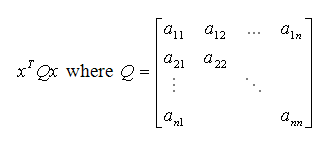
like in MPS files. As symmetry is always assumed, aij=aji for all index pairs (i,j).
Convexity
A fundamental property for nonlinear optimization problems, thus in QCQP as well, is convexity. A region is called convex if for any two points from the region the connecting line segment is also part of the region.
The lack of convexity may give rise to several unfavorable model properties. Lack of convexity in the objective may introduce the phenomenon of locally optimal solutions that are not global ones (a local optimal solution is one for which a neighborhood in the feasible region exists in which that solution is the best). While the lack of convexity in constraints can also give rise to local optima, they may even introduce non–connected feasible regions as shown in Figure Non-connected feasible regions.

Figure 3.1: Non-connected feasible regions
In this example, the feasible region is divided into two parts. In region B, the objective function has two alternative locally optimal solutions, while in region A the objective function is not even bounded.
For convex problems, each locally optimal solution is a global one, making the characterization of the optimal solution efficient.
Characterizing Convexity in Quadratic Constraints
A quadratic constraint of the form
defines a convex region if and only if Q is a so–called positive semi–definite (PSD) matrix.
A square matrix Q is PSD by definition if for any vector (not restricted to the feasible set of a problem) x it holds that xTQx≥0.
It follows that for greater-than or equal constraints
the negative of Q must be PSD.
A nontrivial quadratic equality constraint (one for which not every coefficient is zero) always defines a nonconvex region (or in other words, if both Q and its negative is PSD, then Q must be equal to the 0 matrix). Therefore, quadratic equality constraints are not allowed by the Optimizer.
Determining whether a matrix is PSD is not always obvious nor trivial. There are certain constructs, however, that can easily be recognized as being non convex:
- the product of two variables, say xy, without having both x2 and y2 present;
- having - x2 in any quadratic expression in a less–than or equal constraint, or having x2 in any greater– than or equal constraint.
© 2001-2020 Fair Isaac Corporation. All rights reserved. This documentation is the property of Fair Isaac Corporation (“FICO”). Receipt or possession of this documentation does not convey rights to disclose, reproduce, make derivative works, use, or allow others to use it except solely for internal evaluation purposes to determine whether to purchase a license to the software described in this documentation, or as otherwise set forth in a written software license agreement between you and FICO (or a FICO affiliate). Use of this documentation and the software described in it must conform strictly to the foregoing permitted uses, and no other use is permitted.