QP

To adapt the model developed in Chapter 2 to the new way of looking at the problem, we need to make the following changes:

• New objective function: mean variance instead of total return.
• The risk-related constraint disappears.
• Addition of a new constraint: target yield.

The new objective function is the mean variance of the portfolio, namely:

where VAR_st is the variance/covariance matrix of all shares. This is a quadratic objective function (an objective function becomes quadratic either when a variable is squared, e.g., frac₁², or when two variables are multiplied together, e.g., frac₁ · frac₂).

The target yield constraint can be written as follows:

The limit on the North-American shares as well as the requirement to spend all the money, and the upper bounds on the fraction invested into every share are retained. We therefore obtain the following complete mathematical model formulation:

Implementation with Mosel

In addition to the Xpress Optimizer module mmxprs we now also need to load the module mmnl that adds to the Mosel language the facilities required for the definition of quadratic expressions (mmnl is documented in the `Mosel Language Reference Manual'). We can then use the optimization function maximize (or alternatively minimize) for quadratic objective functions to start the solution process.

This model uses a different data file (folioqp.dat) than the previous models:

           ! trs  haw  thr  tel  brw  hgw  car  bnk  sof  elc
RET: [   (1)   5   17   26   12    8    9    7    6   31   21]

VAR: [ (1 1) 0.1    0    0    0    0    0    0    0    0    0 ! treasury
       (2 1)   0   19   -2    4    1    1    1  0.5   10    5 ! hardware
       (3 1)   0   -2   28    1    2    1    1    0   -2   -1 ! theater
       (4 1)   0    4    1   22    0    1    2    0    3    4 ! telecom
       (5 1)   0    1    2    0    4 -1.5   -2   -1    1    1 ! brewery
       (6 1)   0    1    1    1 -1.5  3.5    2  0.5    1  1.5 ! highways
       (7 1)   0    1    1    2   -2    2    5  0.5    1  2.5 ! cars
       (8 1)   0  0.5    0    0   -1  0.5  0.5    1  0.5  0.5 ! bank
       (9 1)   0   10   -2    3    1    1    1  0.5   25    8 ! software
      (10 1)   0    5   -1    4    1  1.5  2.5  0.5    8   16 ! electronics
     ]

RISK: [2 3 4 9 10]
NA: [1 2 3 4]

Note that we have chosen to use numerical instead of string indices. Since the set SHARES is defined in the model, we do not have to list the index-tuple for every data entry in the file—those tuples given are for clarity's sake only.

model "Portfolio optimization with QP/MIQP"
 uses "mmxprs", "mmnl"              ! Use Xpress Optimizer with QP solver

 parameters
  MAXVAL = 0.3                      ! Max. investment per share
  MINAM = 0.5                       ! Min. investment into N.-American values
  MAXNUM = 4                        ! Max. number of different assets
  TARGET = 9.0                      ! Minimum target yield
 end-parameters

 declarations
  SHARES = 1..10                    ! Set of shares
  RISK: set of integer              ! Set of high-risk values among shares
  NA: set of integer                ! Set of shares issued in N.-America
  RET: array(SHARES) of real        ! Estimated return in investment
  VAR: array(SHARES,SHARES) of real ! Variance/covariance matrix of
                                    ! estimated returns
 end-declarations

 initializations from "folioqp.dat"
  RISK RET NA VAR
 end-initializations

 declarations
  frac: array(SHARES) of mpvar      ! Fraction of capital used per share
 end-declarations

! Objective: mean variance
 Variance:= sum(s,t in SHARES) VAR(s,t)*frac(s)*frac(t)

! Minimum amount of North-American values
 sum(s in NA) frac(s) >= MINAM

! Spend all the capital
 sum(s in SHARES) frac(s) = 1

! Target yield
 sum(s in SHARES) RET(s)*frac(s) >=  TARGET

! Upper bounds on the investment per share
 forall(s in SHARES) frac(s) <= MAXVAL

! Solve the problem
 minimize(Variance)

! Solution printing
 writeln("With a target of ", TARGET, " minimum variance is ", getobjval)
 forall(s in SHARES) writeln(s, ": ", getsol(frac(s))*100, "%")

end-model 

This model (file folioqp.mos) produces the following solution output (tab Output/input of the solution information window):

With a target of 9 minimum variance is 0.5573934236
1: 29.99999999%
2: 7.153923216%
3: 7.382487455%
4: 5.463589348%
5: 12.6553572%
6: 5.911771509%
7: 0.3330412872%
8: 29.99996789%
9: 1.099855797%
10: 6.303833229e-06%

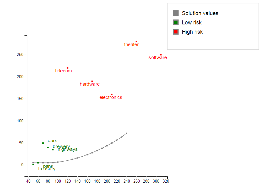
Similarly to the algorithm shown in Chapter 5, we may re-solve this problem with different values of TARGET and plot the results in a target return/standard deviation graph, know as the `efficient frontier' (model file folioqp_graph.mos):

Figure 8.1: Graph of the efficient frontier