Drawing user graphs
In this chapter we show how to draw a user-defined SVG graph. The graph we wish to display is generated as a result of repeated executions of a model with different parameter settings. So we shall first see an example of writing a simple algorithm in the Mosel language involving
- re-definition of constraints,
- repeated re-optimization,
- saving solution information,
- definition of a user graph: drawing points, lines, and texts, and
- simple programming tasks (loops and selections).
Extended problem description
In addition to the data considered so far (see table in Chapter 2), the investor now also has at hand the estimations of the deviations from the expected return per share (Table Estimated deviations). With this additional information, he decides to run the LP model with different limits on the portion of high-risk shares and to represent the results as a graph, plotting the resulting total return against the deviation as a measure of risk.
| Number | Description | Deviation |
|---|---|---|
| 1 | treasury | 0.1 |
| 2 | hardware | 19 |
| 3 | theater | 28 |
| 4 | telecom | 22 |
| 5 | brewery | 4 |
| 6 | highways | 3.5 |
| 7 | cars | 5 |
| 8 | bank | 0.5 |
| 9 | software | 25 |
| 10 | electronics | 16 |
Looping over optimization
We are going to modify the model foliodata.mos from the previous chapter in such a way that the problem is re-optimized repeatedly with different limits on the percentage of high-risk values.
In detail, the model will be transformed to implement the following algorithm:
- Definition of the part of the model that remains unchanged by the parameter changes.
- For every parameter value:
- Re-define the constraint limiting the percentage of high-risk values.
- Solve the resulting problem.
- If the problem is feasible: store the solution values.
- Draw the result graph.
To store the solution value and the total estimated deviation of the result after each optimization run, we declare the following two arrays:
 declarations
  SOLRET: array(range) of real       ! Solution values (total return)
  SOLDEV: array(range) of real       ! Solution values (average deviation)
 end-declarations
The following code fragment introduces a loop around the definition of the constraint limiting the portion of high-risk shares and the solution procedure. To be able to override its previous definition at every iteration, we now give this constraint a name, Risk. If the constraint did not have a name, then each time the loop was executed, a new constraint would be added, and the existing constraint would not be replaced.
 ct:=0
 forall(r in 0..20) do
  ! Limit the percentage of high-risk values
   Risk:= sum(s in RISK) frac(s) <= r/20

   maximize(Return)                  ! Solve the problem
   if (getprobstat = XPRS_OPT) then  ! Save the optimal solution value
    ct+=1
    SOLRET(ct):= getobjval
    SOLDEV(ct):= getsol(sum(s in SHARES) DEV(s)*frac(s))
   else
    writeln("No solution for high-risk values <= ", 100*r/20, "%")
   end-if
 end-do
Above we have used the second form of the forall loop, namely forall/do. This form must be used when several statements are included in the loop. The loop is terminated by end-do.
Another new feature in this code extract is the if/then/else/end-if statement. We only want to save the values for a problem instance if the optimal solution has been found—the solution status is obtained with function getprobstat and tested whether it is `solved to optimality', represented by the constant XPRS_OPT.
The selection statement has two other forms, if/then/end-if and if/then/elif/then/ else/end-if where elif/then may be repeated several times.
For further examples and a complete description of all loops and selection statements available in Mosel the reader is refered to the `Mosel User Guide'.
Drawing a user graph
We now have gathered all the data required to draw the graph. Graphing functions are provided by the module mmsvg (documented in the `Mosel Language Reference Manual'), so it needs to be loaded at the beginning of the model by adding the following line:
uses "mmsvg"
Then the following lines draw the graph (note the use of the sum operator to create a list of points):
 svgaddgroup("GrS", "Solution values", SVG_GREY)
 forall(r in 1..ct) svgaddpoint("GrS", SOLRET(r), SOLDEV(r))
 svgaddline("GrS", sum(r in 1..ct) [SOLRET(r), SOLDEV(r)])
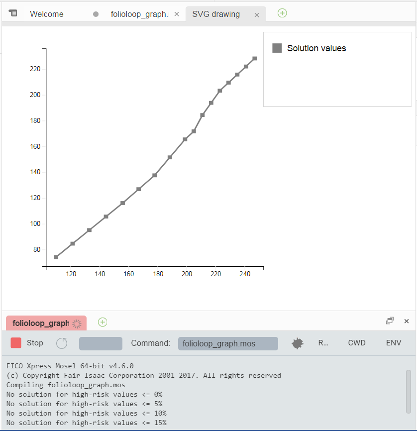
The user graph will be displayed in the editor window of the Workbench workspace. Select the tab SVG drawing to move it to the foreground. With the above we obtain the following output (due to the interplay of the various constraints the resulting graph is not a straight line as one might have expected at first thought):

Figure 6.1: Plot of the result graph
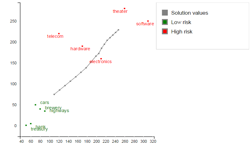
In addition to this graph, we may also display labeled points representing the input data (`GrL' for low risk shares and `GrH' for high risk shares):
 svgaddgroup("GrL", "Low risk", SVG_GREEN)
 svgaddgroup("GrH", "High risk", SVG_RED)

 forall(s in SHARES - RISK) do
  svgaddpoint("GrL", RET(s), DEV(s))
  svgaddtext("GrL", RET(s)+1, 1.3*(DEV(s)-1), s)
 end-do

 forall(s in RISK) do
  svgaddpoint("GrH", RET(s), DEV(s))
  svgaddtext("GrH", RET(s)-2.5, DEV(s)-1, s)
 end-do
Notice the set notation: SHARES - RISK means `all elements of SHARES that are not contained in RISK'.
The complete output now is:

Figure 6.2: Plot of result graph and data
Complete example
The complete model file folioloop_graph.mos with all the features discussed in this chapter looks as follows. Notice that the two modules mmxprs and mmive may be loaded with a single uses statement. The deviation data may either be added to the original data file or, as shown here, read from a second file.
model "Portfolio optimization with LP"
 uses "mmxprs", "mmsvg"             ! Use Xpress Optimizer with SVG graphing

 parameters
  DATAFILE= "folio.dat"             ! File with problem data
  DEVDATA= "foliodev.dat"           ! File with deviation data
  MAXVAL = 0.3                      ! Max. investment per share
  MINAM = 0.5                       ! Min. investment into N.-American values
 end-parameters

 declarations
  SHARES: set of string             ! Set of shares
  RISK: set of string               ! Set of high-risk values among shares
  NA: set of string                 ! Set of shares issued in N.-America
  RET: array(SHARES) of real        ! Estimated return in investment
  DEV: array(SHARES) of real        ! Standard deviation
  SOLRET: array(range) of real      ! Solution values (total return)
  SOLDEV: array(range) of real      ! Solution values (average deviation)
 end-declarations

 initializations from DATAFILE
  RISK RET NA
 end-initializations

 initializations from DEVDATA
  DEV
 end-initializations

 declarations
  frac: array(SHARES) of mpvar      ! Fraction of capital used per share
  Return, Risk: linctr              ! Constraint declaration (optional)
 end-declarations

! Objective: total return
 Return:= sum(s in SHARES) RET(s)*frac(s)

! Minimum amount of North-American values
 sum(s in NA) frac(s) >= MINAM

! Spend all the capital
 sum(s in SHARES) frac(s) = 1

! Upper bounds on the investment per share
 forall(s in SHARES) frac(s) <= MAXVAL

! Solve the problem for different limits on high-risk shares
 ct:=0
 forall(r in 0..20) do
  ! Limit the percentage of high-risk values
   Risk:= sum(s in RISK) frac(s) <= r/20

   maximize(Return)                  ! Solve the problem

   if (getprobstat = XPRS_OPT) then  ! Save the optimal solution value
    ct+=1
    SOLRET(ct):= getobjval
    SOLDEV(ct):= getsol(sum(s in SHARES) DEV(s)*frac(s))
   else
    writeln("No solution for high-risk values <= ", 100*r/20, "%")
   end-if
 end-do

! Drawing a graph to represent results (`GrS') and data (`GrL' & `GrH')
 svgaddgroup("GrS", "Solution values", SVG_GREY)
 svgaddgroup("GrL", "Low risk", SVG_GREEN)
 svgaddgroup("GrH", "High risk", SVG_RED)

 forall(r in 1..ct) svgaddpoint("GrS", SOLRET(r), SOLDEV(r))
 svgaddline("GrS", sum(r in 1..ct) [SOLRET(r), SOLDEV(r)])

 forall(s in SHARES - RISK) do
  svgaddpoint("GrL", RET(s), DEV(s))
  svgaddtext("GrL", RET(s)+1, 1.3*(DEV(s)-1), s)
 end-do

 forall(s in RISK) do
  svgaddpoint("GrH", RET(s), DEV(s))
  svgaddtext("GrH", RET(s)-2.5, DEV(s)-1, s)
 end-do

! Scale the size of the displayed graph
 svgsetgraphscale(10)
 svgsetgraphpointsize(2)

! Optionally save graphic to file
 svgsave("foliograph.svg")

! Display the graph and wait for window to be closed by the user
 svgrefresh
 svgwaitclose

end-model
The problem is not feasible for small limit values on the constraint Risk. Besides the graphs we therefore obtain the following text output:
No solution for high-risk values <= 0%
No solution for high-risk values <= 5%
No solution for high-risk values <= 10%
No solution for high-risk values <= 15%

