Inputting and solving a Linear Programming problem

In this chapter we take the example formulated in Chapter 2 and show how to transform it into a Mosel model which is solved as an LP using Xpress Workbench. More precisely, this involves the following steps:

• starting up Xpress Workbench,
• creating and saving the Mosel file,
• using the Mosel language to enter the model,
• correcting errors and debugging the model,
• solving the model and understanding the displays in Workbench,
• viewing and verifying the solution and understanding the solution in terms of the real world problem instance.

Chapter 10 shows how to formulate and solve the same example with BCL and in Chapter 15 the problem is input and solved directly with Xpress Optimizer.

Starting up Xpress Workbench and creating a new model

We shall develop and execute our Mosel model with the graphical environment Xpress Workbench. If you have followed the standard installation procedure for Xpress, start the program;

• In Windows, double click the Workbench icon on the desktop or select Start » Programs » FICO » Xpress » Xpress Workbench. Otherwise, you can start up Workbench by typing xpworkbench at the command prompt.
• On the Mac, you may have created a shortcut during the installation by dragging the Workbench icon to the Dock. Otherwise, type 'Workbench' into Spotlight, or open Applications » FICO Xpress and double click the Xpress Workbench icon.

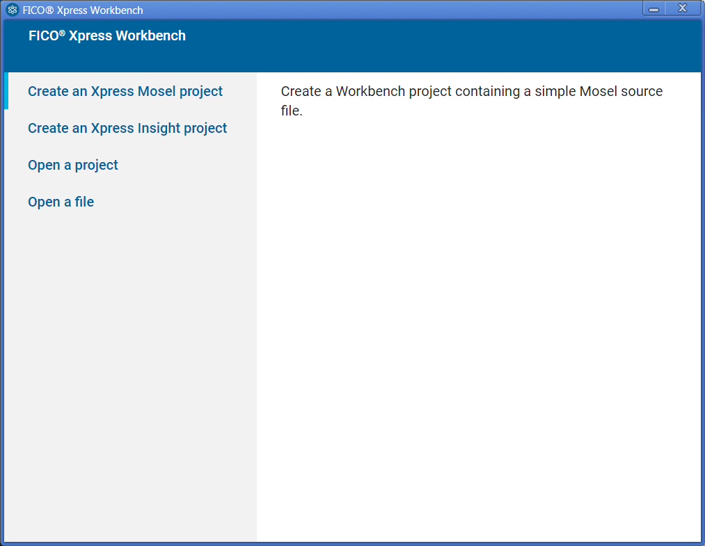
Figure 4.1: Workbench at startup

If you are starting Workbench without having selected any Mosel model you will see the following entry screen where you need to select the option Create an Xpress Mosel project. You will be prompted for location where to create the project. Browse to the desired location, then select the button Make New Folder and enter the name Folio. After confirming with OK you will see the welcome page of the Workbench workspace.

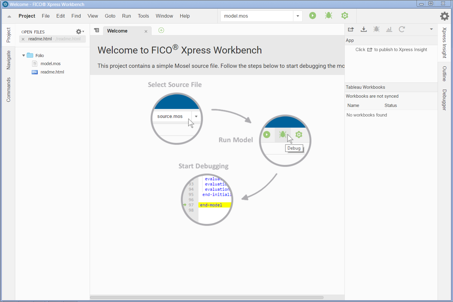
Figure 4.2: Workbench welcome page

Note: If you have started Workbench by selecting a model file this file is opened in the central editor window and the directory listing on its left lists all files in the same location.

The Xpress Workbench workspace window is subdivided into several panes:

At the top, we have the menu and tool bars. The central are is the editor window where the working file will be displayed, and at its bottom opens the logging window during model execution. The window on the left is the project navigation and command history, and the right window contains the debugger and Xpress Insight panes. You may configure the windows displayed via the Window menu.

To create a new model file select File » New From Template » Mosel file or alternatively, double click on the template file model.mos in the directory listing on the left to open it in the central editor window. Select File » Save As... and enter foliolp.mos as the name of the new file. Click Save to confirm your choice. The central window of Workbench is now ready for you to enter the model into the displayed model input template.

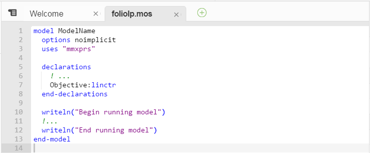
Figure 4.3: Mosel model template

LP model

The mathematical model in the previous chapter may be transformed into the following Mosel model entered into Workbench:

model "Portfolio optimization with LP"
 uses "mmxprs"                       ! Use Xpress Optimizer

 declarations
  SHARES = 1..10                     ! Set of shares
  RISK = {2,3,4,9,10}                ! Set of high-risk values among shares
  NA = {1,2,3,4}                     ! Set of shares issued in N.-America
  RET: array(SHARES) of real         ! Estimated return in investment

  frac: array(SHARES) of mpvar       ! Fraction of capital used per share
 end-declarations

 RET:: [5,17,26,12,8,9,7,6,31,21]

! Objective: total return
 Return:= sum(s in SHARES) RET(s)*frac(s)

! Limit the percentage of high-risk values
 sum(s in RISK) frac(s) <= 1/3

! Minimum amount of North-American values
 sum(s in NA) frac(s) >= 0.5

! Spend all the capital
 sum(s in SHARES) frac(s) = 1

! Upper bounds on the investment per share
 forall(s in SHARES) frac(s) <= 0.3

! Solve the problem
 maximize(Return)

! Solution printing
 writeln("Total return: ", getobjval)
 forall(s in SHARES) writeln(s, ": ", getsol(frac(s))*100, "%")

end-model

Let us now try to understand what we have just written.

General structure

Every Mosel program starts with the keyword model, followed by a model name chosen by the user. The Mosel program is terminated with the keyword end-model.

All objects must be declared in a declarations section, unless they are defined unambiguously through an assignment. For example,

 Return:= sum(s in SHARES) RET(s)*frac(s)

defines Return as a linear constraint and assigns to it the expression

 sum(s in SHARES) RET(s)*frac(s)

There may be several such declarations sections at different places in a model.

In the present case, we define three sets, and two arrays:

• SHARES is a so-called range set—i.e., a set of consecutive integers (here: from 1 to 10).
• RISK and NA are simply sets of integers.
• RET is an array of real values indexed by the set SHARES, its values are assigned after the declarations.
• frac is an array of decision variables of type mpvar, also indexed by the set SHARES. These are the decision variables in our model.

The model then defines the objective function, two linear inequality constraints and one equality constraint and sets upper bounds on the variables.

As in the mathematical model, we use a forall loop to enumerate all the indices in the set SHARES.

Solving

With the procedure maximize, we call Xpress Optimizer to maximize the linear expression Return. As Mosel is itself not a solver, we specify that Xpress Optimizer is to be used with the statement

 uses "mmxprs"

at the begin of the model (the module mmxprs is documented in the `Mosel Language Reference Manual').

Instead of defining the objective function Return separately, we could just as well have written

 maximize(sum(s in SHARES) RET(s)*frac(s))

Output printing

The last two lines print out the value of the optimal solution and the solution values for all variables.

To print an additional empty line, simply type writeln (without arguments). To write several items on a single line use write instead of writeln for printing the output.

Formating

Indentation, spaces, and empty lines in our model have been added to increase readability. They are skipped by Mosel.

Line breaks: It is possible to place several statements on a single line, separating them by semicolons, like

 RISK = {2,3,4,9,10}; NA = {1,2,3,4}

But since there are no special `line end' or continuation characters, every line of a statement that continues over several lines must end with an operator (+, >=, etc.) or characters like `,' that make it obvious that the statement is not terminated.

As shown in the example, single line comments in Mosel are preceded by !. Comments over multiple lines start with (! and terminate with !).

Correcting errors and debugging a model

Having entered the model printed in the previous section, we now wish to execute it, that is, solve the optimization problem and retrieve the results. Choose Run » Run foliolp.mos or alternatively, click on the run button: making sure that the desired model filename is selected in the dropdown box next to it.

At a first attempt to run a model, you are likely to see the message `Compilation failed. Please check for errors.' The bottom window displays the error messages generated by Mosel, for instance as shown in the following figure (Figure Logging output with error messages).

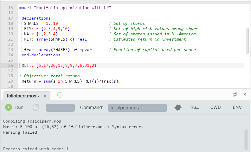
Figure 4.4: Logging output with error messages

When typing in the model from the previous section (there printed in its correct form), we have deliberately introduced some common mistakes that we shall now correct—see the example file foliolperr.mos for the erroneous model.

The first message:

 Mosel: E-100 at (26,32) of `foliolperr.mos': Syntax error.

takes us to the line

 RET:: [5,17,26,12,8,9,7,6,31,21

We need to add the closing bracket to terminate the definition of RET (if the definition continues on the next line, we need to add a comma at the end of this line to indicate continuation).

The next messages that appear after re-running the model:

 Mosel: E-100 at (29,9) of `foliolperr.mos': Syntax error before `='.
 Mosel: E-123 at (29,9) of `foliolperr.mos': `Return' is not defined.
 Mosel: E-124 at (29,42) of `foliolperr.mos': An expression cannot be used as a statement.

take us to the line

 Return = sum(s in SHARES) RET(s)*frac(s)

Finding the error here requires taking a very close look: instead of := we have used =. Since Return should have been defined by assigning it the sum on the right side, this statement now does not have any meaning.

After correcting this error, we try to run the model again, but we are still left with one error message:

 Mosel: E-123 at (44,17) of `foliolperr.mos': `maximize' is not defined.

located in the line

 maximize(Return)

The procedure maximize is defined in the module mmxprs but we have forgotten to add the line

 uses "mmxprs"

at the beginning of the Mosel model. After adding this line, the model compiles correctly.

If you do not remember the correct name of a Mosel keyword while typing in a model, then you may use the code completion feature of the Workbench editor: while you are typing the editor brings up a list of suggestions with Mosel keywords and subroutines.

Debugging

If a model is correct from Mosel's point of view, this does of course not guarantee that it really does what we would like it to do. For instance, we may have forgotten to initialize data, or variables and constraints are not created correctly (they may be part of complex expressions, including logical tests etc.). To check what has indeed been generated by Mosel, we may pause the execution of the model immediately before it terminates by running the model in debug mode: select button to run the model. The model will pause on the last statement to allow you to inspect the model entities in the Debugger window on the right side of the workspace window. Expand the entries under the heading Variables to view the definitions of individual model objects.

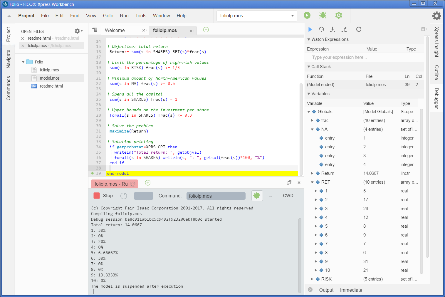
Figure 4.5: Workbench debugger

If you wish to display or trace the values of model entities at other locations you can set breakpoints by clicking onto the grey area in front of the line numbers and re-run the model in debug mode.

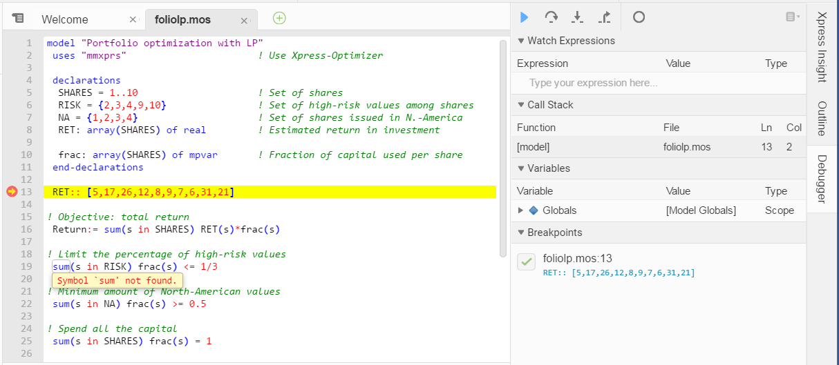
Figure 4.6: Debug run with breakpoint

The debugger controls at the top of the Debugger window (step over: , step into: , step out: ) allow you to step through the model line-by-line or resume/pause its execution ().

Solving and viewing the solution

As mentioned in the previous section, to execute our model we have to select Run » Run foliolp.mos or alternatively, click on the run button: After the successful execution of our model the screen display changes to the following (Figure Display after model execution).

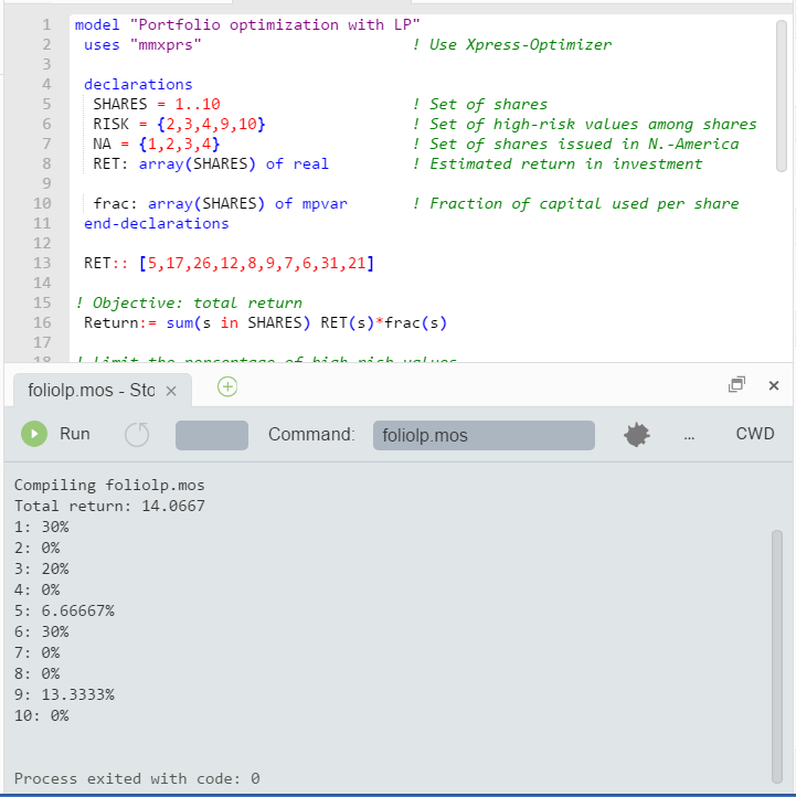
Figure 4.7: Display after model execution

The bottom window contains the log of the Mosel execution and if running in debug mode the left window displays all model entities. Choose the icon window to toggle full-screen display of the output printed by our program:

Total return: 14.0667
1: 30%
2: 0%
3: 20%
4: 0%
5: 6.66667%
6: 30%
7: 0%
8: 0%
9: 13.3333%
10: 0%

This means, that the maximum return of 14.0667 is obtained with a portfolio consisting of shares 1, 3, 5, 6, and 9. 30% of the total amount are spent in shares 1 and 6 each, 20% in 3, 13.3333% in 9 and 6.6667% in 5. It is easily verified that all constraints are indeed satisfied: we have 50% of North-American shares (1 and 3) and 33.33% of high-risk shares (3 and 9).

Now add the line

 setparam("XPRS_VERBOSE", true)

into you model before the call to maximize and re-run it. You will now see more detailed solution information than what is printed by our model (Figure Solver log gdisplay). The upper part of the log contains some statistics about the matrix, in its original and in presolved form (presolving a problem means applying some numerical methods to simplify or transform it). The center part tells us which LP algorithm has been used (Simplex), and the number of iterations and total time needed by the algorithm. Since this problem is very small, it is solved almost instantaneously. After the solver log you see as before the output produced by your model.

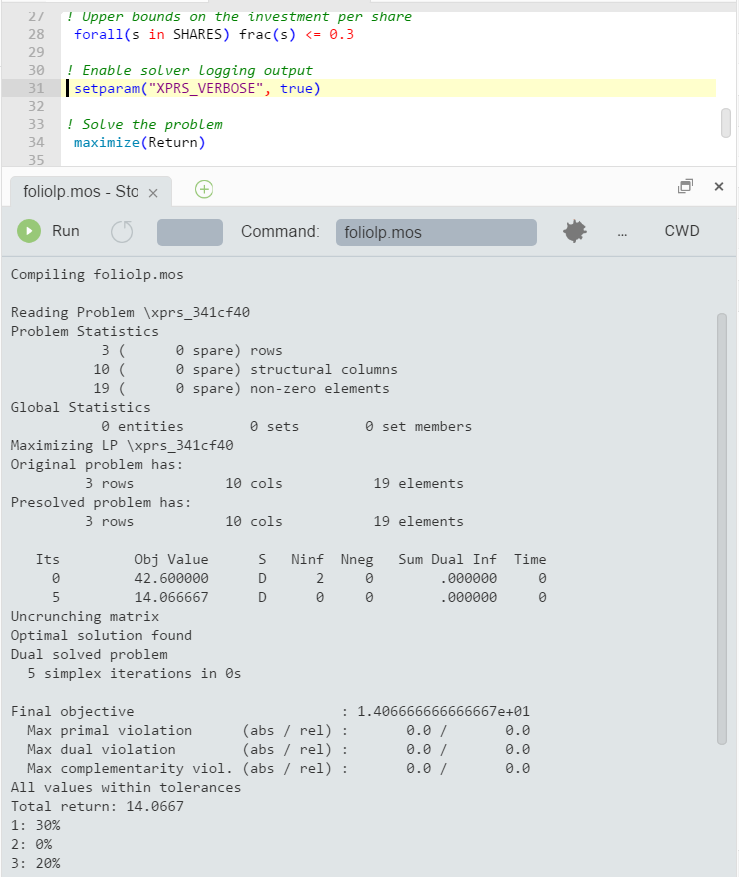
Figure 4.8: Solver log gdisplay

String indices

To make the output of the model more easily understandable, it may be a good idea to replace the numerical indices by string indices.

In our model, we replace the three declaration lines

  SHARES = 1..10
  RISK = {2,3,4,9,10}
  NA = {1,2,3,4}

by the following lines:

  SHARES = {"treasury", "hardware", "theater", "telecom", "brewery",
            "highways", "cars", "bank", "software", "electronics"}
  RISK = {"hardware", "theater", "telecom", "software", "electronics"}
  NA = {"treasury", "hardware", "theater", "telecom"}

And in the initialization of the array RET we now need to use the indices:

 RET::(["treasury", "hardware", "theater", "telecom", "brewery",
        "highways", "cars", "bank", "software", "electronics"])[
	5,17,26,12,8,9,7,6,31,21]

No other changes in the model are required. We save the modified model as foliolps.mos.

The solution output then prints as follows which certainly makes the interpretation of the result easier and more immediate:

Total return: 14.0667
treasury: 30%
hardware: 0%
theater: 20%
telecom: 0%
brewery: 6.66667%
highways: 30%
cars: 0%
bank: 0%
software: 13.3333%
electronics: 0%

Of course, the entity display also works with these string names:

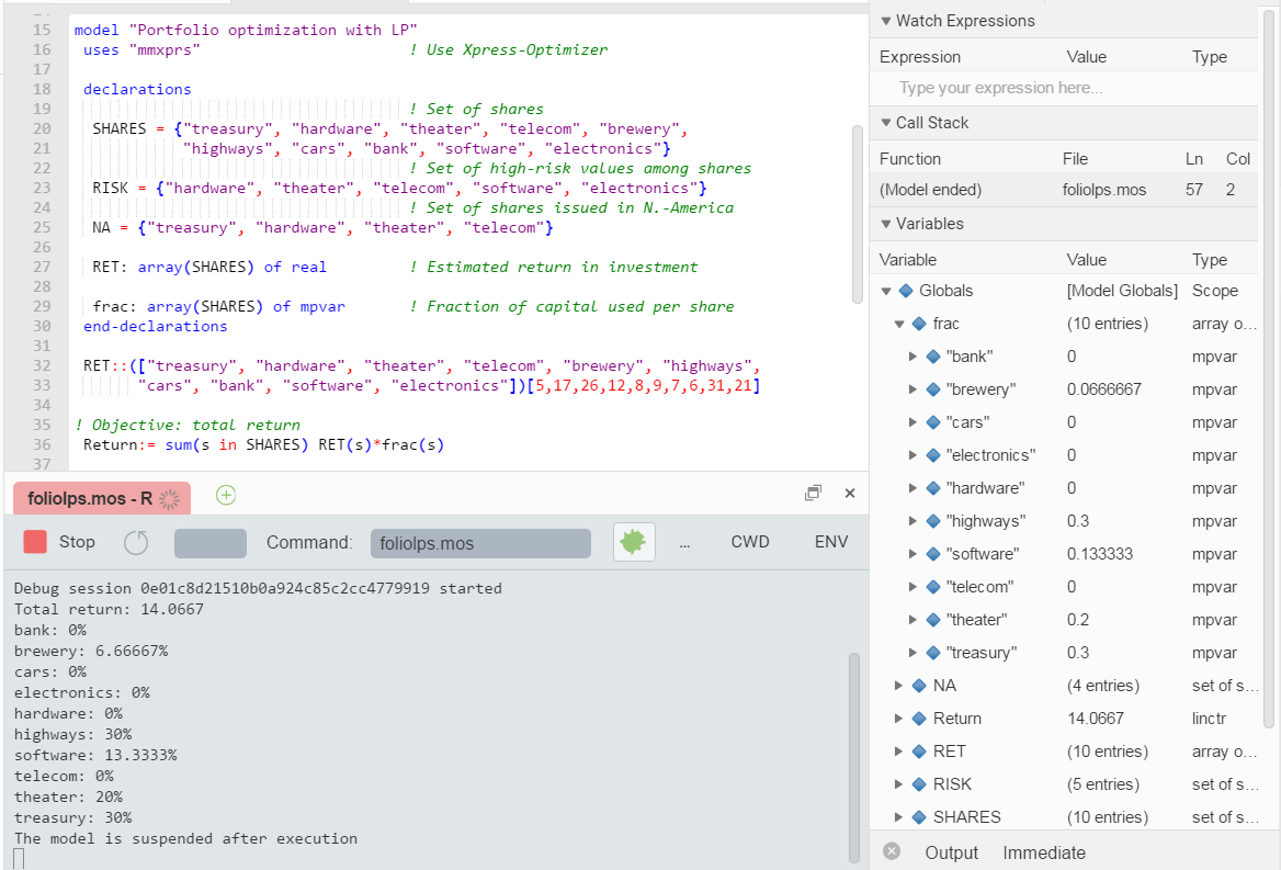
Figure 4.9: Entity display