MIP formulations using other entities

Topics covered in this section:

In principle, all you need in building MIP models are continuous variables and binary variables. But it is convenient to extend the set of modeling entities to embrace objects that frequently occur in practice.

Integer decision variables

values 0, 1, 2, ... up to small upper bound
model discrete quantities
try to use partial integer variables instead of integer variables with a very large upper bound

Semi-continuous variable

may be zero, or any value between the intermediate bound and the upper bound
Semi-continuous integer variables also available: may be zero, or any integer value between the intermediate bound and the upper bound

Special ordered sets

set of decision variables
each variable has a different ordering value, which orders the set
Special ordered sets of type 1 (SOS1): at most one variable may be non-zero
Special ordered sets of type 2 (SOS2): at most two variables may be non-zero; the non-zero variables must be adjacent in ordering

Indicator constraints

associate a binary variable with a linear or nonlinear constraint
model an implication: the constraint is active only if the condition is true

General constraints

specific constraint relations that are recognized by MIP solvers
piecewise linear: can be used in place of SOS-2 formulations
absolute value, minimum value, maximum value of discrete or continuous decision variables
logical constraints: 'and' and 'or' over binary variables

Batch sizes

Must deliver in batches of 10, 20, 30, ...

Decision variables

nship number of batches delivered: integer

ship quantity delivered: continuous
Constraint formulation

ship = 10 · nship

nship	number of batches delivered: integer
ship	quantity delivered: continuous

ship = 10 · nship

Ordered alternatives

Suppose you have N possible investments of which at most one can be selected. The capital cost is CAP_i and the expected return is RET_i.

Often use binary variables to choose between alternatives. However, SOS1 are more efficient to choose between a set of graded (ordered) alternatives.
Define a variable d_i to represent the decision, d_i = 1 if investment i is picked
Binary variable (standard) formulation

d_i : binary variables

Maximize: ret = ∑_i RET_i·d_i

∑_i d_i ≤ 1

∑_i CAP_i·d_i ≤ MAXCAP
SOS1 formulation

{d_i; ordering value CAP_i} : SOS1

Maximize: ret = ∑_i RET_i·d_i

∑_i d_i ≤ 1

∑_i CAP_i·d_i ≤ MAXCAP

Maximize: ret = ∑_i RET_i·d_i
∑_i d_i ≤ 1
∑_i CAP_i·d_i ≤ MAXCAP

Maximize: ret = ∑_i RET_i·d_i
∑_i d_i ≤ 1
∑_i CAP_i·d_i ≤ MAXCAP

Special ordered sets in Mosel

special ordered sets are a special type of linear constraint
the set includes all variables in the constraint
the coefficient of a variable is used as the ordering value (i.e., each value must be unique)

declarations
  I=1..4
  d: array(I) of mpvar
  CAP: array(I) of real
  My_Set, Ref_row: linctr
end-declarations

My_Set:= sum(i in I) CAP(i)*d(i) is_sos1

or alternatively (must be used if a coefficient is 0):

Ref_row:= sum(i in I) CAP(i)*d(i)
makesos1(My_Set, union(i in I) {d(i)}, Ref_row)

Special ordered sets in the Python API

special ordered sets are defined as constraints, specifying the set type ('1' or '2'), a list of variables and the corresponding weight coefficients

import xpress as xp

I = range(4)
CAP = [10, 20, 100, 250]

p = xp.problem()

# Create the decision variables
d = [prob.addVariable(name="d_{}".format(i)) for i in I]

# Define a SOS-1 with weights CAP
p.addSOS(d, CAP, name="My_Set", type=1)

Special ordered sets in the C++ API

special ordered sets are defined as constraints, specifying the set type ('SOS1' or 'SOS2'), a list of variables and the corresponding weight coefficients

static std::vector<int> I = {0, 1, 2, 3};
int main()
{
  XpressProblem prob;
  std::vector<double> CAP = {10, 20, 100, 250};

  // Create the decision variables
  auto d = prob.addVariables(I.size()).withName("d_%d").toArray();

  // Define a SOS-1 with weights CAP
  prob.addConstraint(SOS::sos(SetType::SOS1, d, CAP, "My_Set"));

Price breaks

All items discount

All items discount: when buying a certain number of items we get discounts on all items that we buy if the quantity we buy lies in certain price bands.


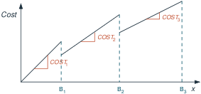
less than B₁	COST₁ each
≥ B₁ and < B₂	COST₂ each
≥ B₂ and < B₃	COST₃ each

Formulation with binary variables or Special Ordered Sets of type 1 (SOS1):

Define binary variables b_i (i=1,2,3), where b_i is 1 if we pay a unit cost of COST_i.
Real decision variables xp_i represent the number of items bought at price COST_i.
The quantity bought is given by x= ∑_ixp_i , with a total price of ∑_iCOST_i·xp_i
MIP formulation :

∑_i b_i = 1

xp₁ ≤ B₁· b₁

B_i-1· b_i ≤ xp_i ≤ B_i· b_i for i=2,3

where the variables b_i are either defined as binaries, or they form a Special Ordered Set of type 1 (SOS1), where the order is given by the values of the breakpoints B_i.

∑_i b_i = 1
xp₁ ≤ B₁· b₁
B_i-1· b_i ≤ xp_i ≤ B_i· b_i for i=2,3

Formulation as piecewise linear expression:

Specification as list of piecewise linear segments with associated intervals:


⋃_i=1,2,3 [B_i-1,B_i[ : COST_i·x

TotalCost:= pwlin(union(i in 1..3) [pws(B(i-1), COST(i)*x)])

totalcost = xp.pwl({(B[i-1],B[i]): COST[i]*x[i] for i in range(1,3)})

Specification as list of points:


⋃_i=1,2,3 [B_i-1,COST_i·B_i-1,B_i,COST_i·B_i]

TotalCost:= pwlin(x, union(i in 1..3) [B(i-1), COST(i)*B(i-1), B(i), COST(i)*B(i)])

In Python, it is possible to specify piecewise linear functions as a list of points using the problem.addpwlcons method. The example assumes that B and COST are array (lists) containing the x-values and y-values of the breakpoints, respectively.

prob.addpwlcons([x], [totalcost], [0], B, COST)

Variable x = prob.addVariable();
Variable fx = prob.addVariable();
std::vector<double> B = ...;
std::vector<double> COST = ...;
std::vector<double> breakX = {0, B[0], B[0], B[1], B[1], B[2]};
std::vector<double> breakY = {0, B[0]*COST[0], B[0]*COST[1], B[1]*COST[1],
                              B[1]*COST[2], B[2]*COST[2]};
prob.addConstraint(fx.pwlOf(x, breakX, breakY));

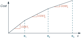
Incremental pricebreaks

Incremental pricebreaks: when buying a certain number of items we get discounts incrementally. The unit cost for items between 0 and B₁ is COST₁, items between B₁ and B₂ cost COST₂ each, etc.

Formulation with Special Ordered Sets of type 2 (SOS2):

Associate real valued decision variables w_i (i=0,1,2,3) with the quantity break points B₀ = 0, B₁, B₂ and B₃.
Cost break points CBP_i (=total cost of buying quantity B_i):

CBP₀=0

CBP_i = CBP_i-1+COST_i· (B_i-B_i-1) for i=1,2,3
Constraint formulation:

∑_iw_i=1

TotalCost = ∑_i CBP_i· w_i

x = ∑_i B_i· w_i

where the w_i form a SOS2 with reference row coefficients given by the coefficients in the definition of the total amount x.
For a solution to be valid, at most two of the w_i can be non-zero, and if there are two non-zero they must be contiguous, thus defining one of the line segments.

CBP₀=0
CBP_i = CBP_i-1+COST_i· (B_i-B_i-1) for i=1,2,3

∑_iw_i=1
TotalCost = ∑_i CBP_i· w_i
x = ∑_i B_i· w_i

is_sos2 cannot be used here due to the 0-valued coefficient of w₀

  Defx := x = sum(i in 1..3) B(i)*w(i)
  makesos2(My_Set, union(i in 0..3) {w(i)}, Defx)
  sum(i in 1..3) w(i) = 1

p.addSOS(w, B, type=2)
p.addConstraint(xp.Sum(w) == 1)

  std::vector<int> I = {0, 1, 2};
  std::vector<double> B = ...;
  auto x = prob.addVariable();
  auto w = prob.addVariables(I.size()).withName("w_%d").toArray();
  prob.addConstraint(SOS::sos(SetType::SOS2, w, B, "Defx"));
  prob.addConstraint(sum(I, [&](auto i) { return w[i];}) == 1.0);

Formulation using binaries:

Define binary variables b_i (i=1,2,3), where b_i is 1 if we have bought any items at a unit cost of COST_i.
Real decision variables xp_i (i=1,..3) for the number of items bought at price COST_i.
Total amount bought: x = ∑_i xp_i
Constraint formulation:

(B_i-B_i-1)· b_i+1 ≤ xp_i ≤ (B_i-B_i-1)· b_i for i=1,2

xp₃ ≤ (B₃-B₂)· b₃

b₁ ≥ b₂ ≥ b₃

(B_i-B_i-1)· b_i+1 ≤ xp_i ≤ (B_i-B_i-1)· b_i for i=1,2
xp₃ ≤ (B₃-B₂)· b₃
b₁ ≥ b₂ ≥ b₃

Formulation as piecewise linear expression:

Specification as list of slopes with associated intervals:

⋃_i=1,2,3 [B_i-1,B_i[ : COST_i
Only points of slope changes are specified, start value is 0
```
TotalCost:= pwlin(x, union(i in 1..2) [B(i)], union(i in 1..3) [COST(i)])
```
Python does not support specifying piecewise linear functions as a list of slopes

⋃_i=1,2,3 [B_i-1,B_i[ : COST_i

Specification as list of piecewise linear segments with associated intervals:


⋃_i=1,2,3 [B_i-1,B_i[ : CBP_i-1+COST_i·(x-B_i-1)

TotalCost:= pwlin(union(i in 1..3) [pws(B(i-1), CBP(i-1)+COST(i)*(x-B(i-1)))])

totalcost = xp.pwl({(B[i-1],B[i]): COST[i-1]+COST[i]*(x[i]-B[i-1])) for i in range(1,3)})

Specification as list of points:


⋃_i=0,1,2,3 [B_i,CBP_i]

TotalCost:= pwlin(x, union(i in 0..3) [B(i), CBP(i)])

In Python, it is possible to specify piecewise linear functions as a list of points using the problem.addpwlcons method. The example assumes that B and CBP are array (lists) containing the x-values and y-values of the breakpoints, respectively.

prob.addpwlcons([x], [totalcost], [0], B, CBP)

Variable x = prob.addVariable();
Variable fx = prob.addVariable();
int npieces = 3;
std::vector<double> B = ...;
std::vector<double> COST = ...;
std::vector<double> breakX = {0, B[0], B[1], B[2]};
std::vector<double> breakY = {0};
for (int i = 1; i <= npieces; i++)  breakY[i] = breakY[i-1] + COST[i-1]*(B[i] - B[i-1]);
prob.addConstraint(fx.pwlOf(x, breakX, breakY));

Non-linear functions

Can model non-linear functions in the same way as incremental pricebreaks

approximate the non-linear function with a piecewise linear function
use an SOS2 to model the piecewise linear function
alternatively, formulate as piecewise linear expression by specifying a list of points
note that certain nonlinear functions (e.g. absolute value, minimum value, maximum value) are recognized by MIP solvers and can be used directly in the formulation of MIP models, see Section General constraints

Non-linear function in a single variable

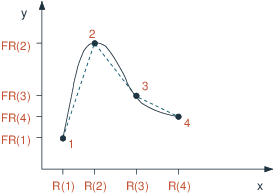
x-coordinates of the points: R₁, ..., R₄
y-coordinates FR₁, ..., FR₄. So point 1 is (R₁,FR₁) etc.
Let weights (decision variables) associated with point i be w_i (i=1,...,4)
Form convex combinations of the points using weights w_i to get a combination point (x,y):

x = ∑_i w_i·R_i

y = ∑_i w_i·FR_i

∑_i w_i = 1

where the variables w_i form an SOS2 set with ordering coefficients defined by values R_i.

x = ∑_i w_i·R_i
y = ∑_i w_i·FR_i
∑_i w_i = 1

Mosel implementation (SOS-2):

 declarations
  I=1..4
  x,y: mpvar
  w: array(I) of mpvar
  R,FR: array(I) of real
 end-declarations

! ...assign values to arrays R and FR...

! Define the SOS-2 with "reference row" coefficients from R
 Defx:= sum(i in I) R(i)*w(i) is_sos2
 sum(i in I) w(i) = 1

! The variable and the corresponding function value we want to approximate
 x = Defx
 y = sum(i in I) FR(i)*w(i)

Mosel implementation (piecewise linear):

 uses "mmxnlp"
 declarations
  I=1..4
  x,y: mpvar
  R,FR: array(I) of real
 end-declarations

! ...assign values to arrays R and FR...

! Define the piecewise linear expression
 y = pwlin(x, sum(i in I) [R(i), FR(i)])

! Only consider the x-values interval defined by the breakpoints
 setrange(x, R(1), R(4))

Python implementation (SOS-2):

import xpress as xp

I = range(4)
R = [1, 2.5, 4.5, 6.5]
FR = [1.5, 6, 3.5, 2.5]

p = xp.problem()

# Create the decision variables
x = p.addVariable(lb=R[0],ub=R[3],name="x") # x-values interval defined by the breakpoints
y = p.addVariable(name="y")
w = [p.addVariable(name="w{0}".format(i)) for i in I]

# Define the SOS-2 with weights R
p.addSOS(w, R, name="Defx", type=2)

# Weights must sum up to 1
p.addConstraint(xp.Sum(w[i] for i in I) == 1.0)

# The variable and the corresponding function value we want to approximate
p.addConstraint(x == xp.Sum(R[i]*w[i] for i in I))
p.addConstraint(y == xp.Sum(FR[i]*w[i] for i in I))
...

C++ implementation (SOS-2):

#include <iostream>
#include <xpress.hpp>
using namespace xpress;
using namespace xpress::objects;
using xpress::objects::utils::sum;
using namespace std;

static std::vector<int> I = {0, 1, 2, 3};

int main()
{
  XpressProblem prob;
  std::vector<double> R = {1, 2.5, 4.5, 6.5};
  std::vector<double> FR = {1.5, 6, 3.5, 2.5};

  // Create the decision variables
  auto x = prob.addVariable(R[0], R[3], ColumnType::Continuous, "x");
                            // x-values interval defined by the breakpoints
  auto y = prob.addVariable("y");
  auto w = prob.addVariables(I.size()).withName("w_%d").toArray();

  // Define the SOS-2 with weights R
  prob.addConstraint(SOS::sos(SetType::SOS2, w, R, "Defx"));

  // Weights must sum up to 1
  prob.addConstraint(sum(I, [&](auto i) { return w[i];}) == 1.0);

  // The variable and the corresponding function value we want to approximate
  prob.addConstraint(x == sum(I, [&](auto i) { return R[i]*w[i];}));
  prob.addConstraint(y == sum(I, [&](auto i) { return FR[i]*w[i];}));
...

Non-linear function in two variables

Interpolation of a function f in two variables: approximate f at a point P by the corners C of the enclosing square of a rectangular grid (NB: the representation of P=(x,y) by the four points C obviously means a fair amount of degeneracy).

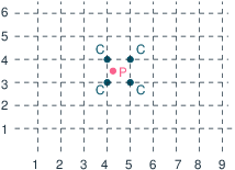
x-coordinates of grid points: X₁, ..., X_n
y-coordinates of grid points: Y₁, ..., Y_m. So grid points are (X_i,Y_j).
Function evaluation at grid points: FXY₁₁, ..., FXY_nm
Define weights (decision variables) associated with x and y coordinates, wx_i respectively wy_j, and for each grid point (X(i),Y(j)) define a variable wxy_ij

Form convex combinations of the points using the weights to get a combination point (x,y) and the corresponding function approximation:


x = ∑_i wx_i·X_i
y = ∑_j wy_j·Y_j
f = ∑_ij wxy_ij·FXY_ij
∀ i=1,...,n: ∑_j wxy_ij = wx_i
∀ j=1,...,m: ∑_i wxy_ij = wy_j
∑_i wx_i = 1
∑_j wy_j = 1

where the variables wx_i form an SOS2 set with ordering coefficients defined by values X_i, and the variables wy_j are a second SOS2 set with coordinate values Y_j as ordering coefficients.

 declarations
  RX,RY:range
  X: array(RX) of real          ! x coordinate values of grid points
  Y: array(RY) of real          ! y coordinate values of grid points
  FXY: array(RX,RY) of real     ! Function evaluation at grid points
 end-declarations

! ... initialize data 

 declarations
  wx: array(RX) of mpvar        ! Weight on x coordinate
  wy: array(RY) of mpvar        ! Weight on y coordinate
  wxy: array(RX,RY) of mpvar    ! Weight on (x,y) coordinates
  x,y,f: mpvar
 end-declarations

! Definition of SOS (assuming coordinate values <>0)
 sum(i in RX) X(i)*wx(i) is_sos2
 sum(j in RY) Y(j)*wy(j) is_sos2

! Constraints 
 forall(i in RX) sum(j in RY) wxy(i,j) = wx(i)
 forall(j in RY) sum(i in RX) wxy(i,j) = wy(j)
 sum(i in RX) wx(i) = 1
 sum(j in RY) wy(j) = 1

! Then x, y and f can be calculated using 
 x = sum(i in RX)  X(i)*wx(i)
 y = sum(j in RY)  Y(j)*wy(j)
 f = sum(i in RX,j in RY) FXY(i,j)*wxy(i,j)

! f can take negative or positive values (unbounded variable)
 f is_free

import xpress as xp

NX = 10
NY = 10
RX = range(NX)
RY = range(NY)

X = [i+1 for i in RX]
Y = [j+1 for j in RY]
FXY = [[(i-4)*(j-4) for i in RX] for j in RY]

p = xp.problem()

# Create the decision variables
x = p.addVariable(name="x")
y = p.addVariable(name="y")
f = p.addVariable(lb=-xp.infinity, ub=xp.infinity, name="f")
wx = [p.addVariable(name="wx_{}".format(i)) for i in RX]
wy = [p.addVariable(name="wy_{}".format(i)) for i in RY]
wxy = [[p.addVariable(name="wxy_{}_{}".format(i,j)) for i in RX] for j in RY]

# Define the SOS-2 for coordinate x 
p.addSOS(wx, X, name="sos_x", type=2)
# Define the SOS-2 for coordinate y 
p.addSOS(wy, Y, name="sos_y", type=2)

# Weights must sum up to 1 along the two coordinates 
p.addConstraint(xp.Sum(wx[i] for i in RX) == 1.0)
p.addConstraint(xp.Sum(wy[j] for j in RY) == 1.0)

# wx, wy and wxy must be consistent
p.addConstraint(wx[i] == xp.Sum(wxy[i][j] for j in  RY) for i in RX)
p.addConstraint(wy[j] == xp.Sum(wxy[i][j] for i in  RX) for j in RY)

# The coordinates and the corresponding function value we want to approximate
p.addConstraint(x == xp.Sum(X[i]*wx[i] for i in RX))
p.addConstraint(y == xp.Sum(Y[j]*wy[j] for j in RY))
p.addConstraint(f == xp.Sum(FXY[i][j]*wxy[i][j] for i in RX for j in RY))

#include <iostream>
#include <xpress.hpp>
using namespace xpress;
using namespace xpress::objects;
using xpress::objects::utils::sum;
using namespace std;

int main()
{
  XpressProblem prob;

  // Problem data
  static const int NX = 10;
  static const int NY = 10;

  std::array<double,NX> X;
  for (int i = 0; i < NX; i++)  X[i] = (double)(i+1);
  std::array<double,NY> Y;
  for (int j = 0; j < NY; j++)  Y[j] = (double)(j+1);
  std::array<std::array<double,NY>, NX> FXY;
  for (int i = 0; i < NX; i++) {
    for (int j = 0; j < NY; j++) {
      FXY[i][j] = (double)(i-4)*(j-4);
    }
  }

  // Create the decision variables
  auto x = prob.addVariable("x");
  auto y = prob.addVariable("y");
  auto f =
    prob.addVariable(XPRS_MINUSINFINITY, XPRS_PLUSINFINITY, ColumnType::Continuous, "f");
  auto wx = prob.addVariables(NX).withName("wx_%d").toArray();
  auto wy = prob.addVariables(NY).withName("wy_%d").toArray();
  auto wxy = prob.addVariables(NX, NY).withName("wxy_%d_%d").toArray();

  // Define the SOS-2 for coordinate x
  prob.addConstraint(SOS::sos(SetType::SOS2, wx, X, "sos_x"));
  // Define the SOS-2 for coordinate y
  prob.addConstraint(SOS::sos(SetType::SOS2, wy, Y, "sos_y"));

  // Weights must sum up to 1 along the two coordinates
  prob.addConstraint(sum(NX, [&](auto i) { return wx[i]; }) == 1.0);
  prob.addConstraint(sum(NY, [&](auto j) { return wy[j]; }) == 1.0);

  // wx, wy and wxy must be consistent
  prob.addConstraints(NX, [&](auto i) {
    return wx[i] == sum(NY, [&](auto j) { return wxy[i][j]; });
  });
  prob.addConstraints(NY, [&](auto j) {
    return wy[j] == sum(NX, [&](auto i) { return wxy[i][j]; });
  });

  // The coordinates and the corresponding function value we want to approximate
  prob.addConstraint(x == sum(NX, [&](auto i) { return X[i]*wx[i]; }));
  prob.addConstraint(y == sum(NY, [&](auto j) { return Y[j]*wy[j]; }));
  prob.addConstraint(f == sum(NX, [&](auto i) {
    return sum(NY, [&](auto j) { return FXY[i][j]*wxy[i][j]; });
  }));
...

Minimum activity level

Continuous production rate make. May be 0 (the plant is not operating) or between allowed production limits MAKEMIN and MAKEMAX

Can impose using a semi-continuous variable: may be zero, or any value between the intermediate bound and the upper bound
Semi-continuous variables are slightly more efficient than the alternative binary variable formulation that we saw before. But if you incur fixed costs on any non-zero activity, you must use the binary variable formulation (see Section Minimum activity level).

make is_semcont MAKEMIN
make <= MAKEMAX

make = p.addVariable(vartype=xp.semicontinuous, threshold=MAKEMIN, ub=MAKEMAX, name="make")

auto make = prob.addVariable(0, MAKEMAX, ColumnType::SemiContinuous, "make");
make.setLimit(MAKEMIN);

Partial integer variables

In general, try to keep the upper bound on integer variables as small as possible. This reduces the number of possible integer values, and so reduces the time to solve the problem.
Sometimes this is not possible – a variable has a large upper bound and must take integer values.
⇒ Try to use partial integer variables instead of integer variables with a very large upper bound: takes integer values for small values, where it is important to be precise, but takes real values for larger values, where it is OK to round the value afterwards.
For example, it may be important to clarify whether the value is 0, 1, 2, ..., 10, but above 10 it is OK to get a real value and round it.

x is_partint 10        ! x is integer valued from 0 to 10
x <= 20                ! x takes real values from 10 to 20

make = p.addVariable(vartype=xp.partiallyinteger, threshold=10, ub=20, name="make")

auto x = prob.addVariable(0, 20, ColumnType::PartialInteger, "x");   // x has upper bound 20
x.setLimit(10);                                          // x is integer valued from 0 to 10

General constraints

Certain nonlinear constraint relations (refered to as general constraints) are recognized by MIP solvers and they are treated as MIP modeling constructs. These include

piecewise linear expressions (see examples in Sections Price breaks and Non-linear functions above)
absolute value, minimum value, maximum value of discrete or continuous decision variables
logical constraints: 'and' and 'or' over binary variables (see Section Boolean variables and logical constraints )

The Mosel implementation of the numerical constraints abs, fmin and fmax makes it possible to use linear expressions as argument to these functions. Note that models using these general constraints need to load the mmxnlp module in addition to mmxprs although the problems will be solved by the Xpress MIP solver.

 uses "mmxnlp"

 public declarations
   R=1..3
   x: array(R) of mpvar
   y,z: mpvar
 end-declarations

 forall(i in R) x(i) <= 20
 abs(x(1)-2*x(2)) <= 10                     ! Absolute value constraint
 MinCtr:= fmin(union(i in R) [x(i)]) >= 5   ! Minimum value constraint
 y = fmax(x(3), 20, x(1)-z)                 ! Maximum value constraint

 maximize(sum(i in R) x(i))                 ! Solve as MIP problem
 if getprobstat=XPRS_OPT then               ! Solution reporting
   writeln("Solution: ", getobjval)
   forall(i in R) write("x", i, "=", x(i).sol, ", ")
   writeln("y=", y.sol, ", z=", z.sol)
   writeln("abs=", getsol(abs(x(1)-2*x(2))), ", Min of x(i)=", MinCtr.sol+5)
 else
   writeln("No solution")
 end-if

The Python implementation of the numerical constraints xp.abs, xp.min and xp.max makes it possible to use linear expressions as argument to these functions.

import xpress as xp

R = range(3)

p = xp.problem()

x = [p.addVariable(name="x_{}".format(i)) for i in R]
y = p.addVariable()
z = p.addVariable()

p.addConstraint(x[i] <= 20 for i in R)
p.addConstraint(xp.abs(x[0] - 2*x[1]) <= 10)      # Absolute value constraint
p.addConstraint(xp.min(x) >= 5)                   # Minimum value constraint
p.addConstraint(y == xp.max(x[2], 20, x[0]-z))    # Maximum value constraint

p.setObjective(xp.Sum(x), sense=xp.maximize)

p.optimize()                                      # Solve as MIP problem

if p.attributes.solstatus in [SolStatus.FEASIBLE",SolStatus."OPTIMAL"]:
    print("Solution:", p.attributes.objval())
    for i in R:
        print(x[i].name,"=",p.getSolution(x[i]))
    print("y=", p.getSolution(y), ", z=", p.getSolution(z))
    print("abs=", p.getSolution(xp.abs(x[0]-2*x[1])), ", Min of x(i)=", min(p.getSolution(x)))
else:
    print("No solution")

The implementation of general constraints with the C++ API introduces auxiliary variables for the formulation of the constraints since absOf/minOf/maxOf are not defined for expressions, they expect decision variables as their arguments.

using namespace xpress;
using namespace xpress::objects;
using xpress::objects::utils::sum;
using namespace std;

int main()
{
  XpressProblem prob;

  // Create the decision variables
  auto x = prob.addVariables(3).withName("x_%d").withUB(20).toArray();
  auto y = prob.addVariable("y");
  auto z = prob.addVariable("z");

  // abs(x_0 - 2*x_1) <= 10
  auto diff1 = prob.addVariable("diff1");
  auto absOfDiff1 = prob.addVariable("absOfDiff1");
  prob.addConstraint(diff1 == x[0] - 2*x[1]);
  prob.addConstraint(absOfDiff1.absOf(diff1));
  absOfDiff1.setUB(10);

  // min(x_i) >= 5
  auto minOfX = prob.addVariable("minOfX");
  prob.addConstraint(minOfX.minOf(x));
  minOfX.setLB(5);

  // y = max(x_2, 20, x_0 - z)
  auto diff2 = prob.addVariable("diff2");
  prob.addConstraint(diff2 == x[0] - z);
  std::array<Variable,2> maxVarArgs = {x[2], diff2};
  prob.addConstraint(y.maxOf(maxVarArgs, 20));

  // Objective
  prob.setObjective(sum(x), ObjSense::Maximize);

  // Solve the problem
  prob.optimize();
...

© 2001-2025 Fair Isaac Corporation. All rights reserved. This documentation is the property of Fair Isaac Corporation (“FICO”). Receipt or possession of this documentation does not convey rights to disclose, reproduce, make derivative works, use, or allow others to use it except solely for internal evaluation purposes to determine whether to purchase a license to the software described in this documentation, or as otherwise set forth in a written software license agreement between you and FICO (or a FICO affiliate). Use of this documentation and the software described in it must conform strictly to the foregoing permitted uses, and no other use is permitted.

Contents

Index

Glossary

Search Results