Deployment to Xpress Insight

Topics covered in this section:

Xpress Insight embeds Python models into a multi-user application for deploying optimization models in a distributed client-server architecture. Through the Xpress Insight GUI, business users interact with Python models to evaluate different scenarios and model configurations without directly accessing to the model itself.

Preparing the model file

For embedding a Python model into Xpress Insight, we need to make a few edits to the Python model in order to establish the connection between Python and Xpress Insight.

Firstly, we need to import the package xpressinsight that provides the required additional functionality, along with other packages needed. Then, the InsightApp class, which contains the model entities and the definition of the two default execution modes (LOAD and RUN), is created following the AppConfig decorator, where the app name and version are defined. Insight entities, i.e. model entities that are meant to be displayed or edited via the UI, are declared within the InsightApp class. By default, model entities are of type INPUT, and are populated during the execution of the LOAD mode. Entities can also be of type RESULT, in which case they should be marked with manage=xi.Manage.RESULT and be populated during the execution of the RUN mode.

Within the InsightApp class, the LOAD mode logic is defined in a function following the ExecModeLoad decorator, while the RUN mode programmatic logic (which contains the statement and solving of the optimization problem) in a function that has been marked with the xpressinsight.ExecModeRun decorator.

The main function creates an instance of the InsightApp class via the create_app method, with its call_exec_modes method allowing for the execution of both the LOAD and RUN modes in test mode.

The resulting Python program named application.py has the following contents—this model can also simply be run standalone, e.g. from Workbench or the Python command line.

import xpressinsight as xi
import xpress as xp
import pandas as pd
import sys

@xi.AppConfig(name="Portfolio optimization", version=xi.AppVersion(1, 0, 0))
class InsightApp(xi.AppBase):
    # Input entities
    MaxHighRisk: xi.types.Param(default=1/3)
    MaxPerShare: xi.types.Param(default=0.3)
    MinNorthAmerica: xi.types.Param(default=0.5)
    ShareIds: xi.types.Index(dtype=xi.string, alias="Shares")

    # Input and result entities indexed over ShareIds
    Shares: xi.types.DataFrame(index="ShareIds", columns=[
        xi.types.Column("Return", dtype=xi.real, alias="Expected Return on Investment"),
        xi.types.Column("HighRisk", dtype=xi.boolean, alias="High-risk value"),
        xi.types.Column("NorthAmerica", dtype=xi.boolean, alias="Issued in North America"),
        xi.types.Column("fraction", dtype=xi.real, alias="Fraction used",
            manage=xi.Manage.RESULT)
    ])

    # Constant class attribute
    DATAFILE = "shares.csv"

    @xi.ExecModeLoad(descr="Load input data and initialize all input entities.")
    def load(self):
        print("Loading data.")
        self.Shares = pd.read_csv(InsightApp.DATAFILE, index_col=['ShareIds'])
        self.ShareIds = self.Shares.index
        print("Loading finished.")

    @xi.ExecModeRun(descr="Solve problem and initialize all result entities.")
    def run(self):
        print('Starting optimization.')

        # Create Xpress problem and variables
        p = xp.problem("portfolio")
        self.Shares['fractionVar'] = pd.Series(p.addVariables(self.ShareIds,
            vartype=xp.continuous, name='fractionVar'))

        # Objective: expected total return
        objective = xp.Sum(self.Shares.Return * self.Shares.fractionVar)
        p.setObjective(objective, sense=xp.maximize)

        # Limit the percentage of high-risk values
        limit_high_risk = \
            xp.Sum(self.Shares.loc[self.Shares.HighRisk, 'fractionVar']) \
            <= self.MaxHighRisk
        p.addConstraint(limit_high_risk)

        # Minimum amount of North-American values
        limit_north_america = \
            xp.Sum(self.Shares.loc[self.Shares.NorthAmerica, 'fractionVar']) \
            >= self.MinNorthAmerica
        p.addConstraint(limit_north_america)

        # Spend all the capital
        p.addConstraint(xp.Sum(self.Shares.fractionVar) == 1)

        # Upper bounds on the investment per share
        p.addConstraint(share.fractionVar <= self.MaxPerShare for share_id,
            share in self.Shares.iterrows())

        # Solve optimization problem
        p.optimize()

        print('Optimization finished.')

if __name__ == "__main__":
    app = xi.create_app(InsightApp)
    sys.exit(app.call_exec_modes(["LOAD", "RUN"]))

Note that we have removed all solution output from this model: we are going to use Xpress Insight for representing the results.

The app archive

Since Xpress Insight executes Python files in a distributed architecture (so, possibly not on the same machine from where the model file is input) we recommend to include any input data files used by the model in the Xpress Insight app archive. The app archive is a ZIP archive that contains the subdirectories model_resources (data files), client_resources (custom view definitions), and python_source (Python model source files). For our example, we create a ZIP archive folioinsight.zip with the data file shares.csv in the subdirectory model_resources.

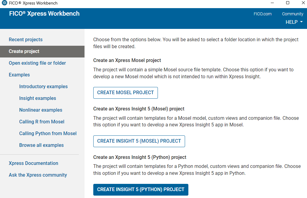
Figure 15.1: Creating a new Insight project

With Xpress Workbench, select the option 'Create project' followed by 'Create Insight (Python) project' at startup to create the directory structure expected by Xpress Insight and replace the template model (in subdirectory python_source), configuration (application.xml and subdirectory client_resources), and data files (in subdirectory model_resources) by the files of your Insight Python project. In order to work with an existing app, select Open existing file or folder followed by Open project when starting up Workbench and browse to the desired folder or double click on a Python file in the source subdirectory and select 'Open Insight app' in the dialog box.

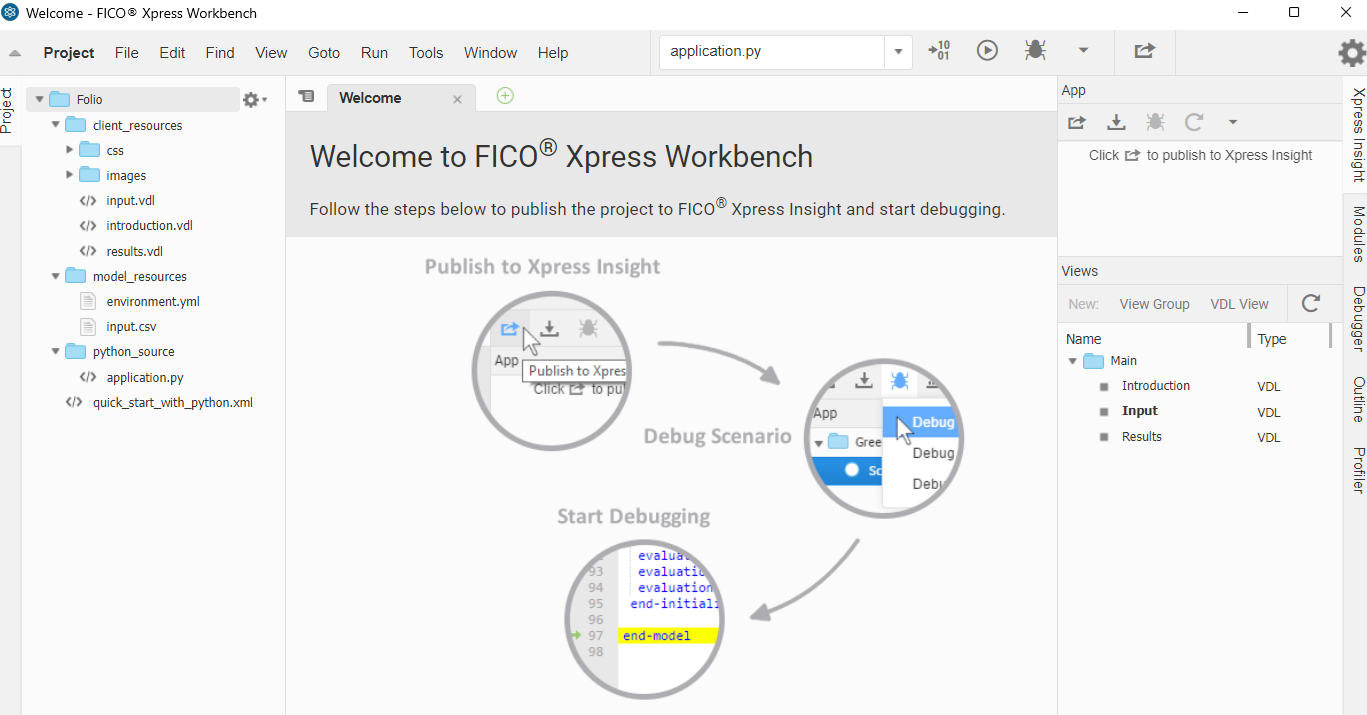
Figure 15.2: Default Xpress Insight Python app template

Select the button to create the app archive or to publish the app directly to Insight. If the app has been published successfully the link 'Open in Xpress Insight' in the green message box will take you to the app loaded in the Insight web client opened with your default web browser.

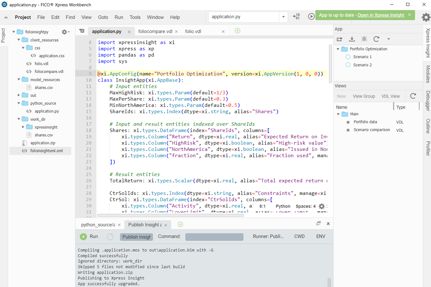
Figure 15.3: Deploying an app to Xpres Insight

Working with the Xpress Insight Web Client

Open the Xpress Insight Web Client by directing your web browser to the Web Client entry page: with a default desktop installation of Xpress Insight this will be the page: http://localhost:8080/insight

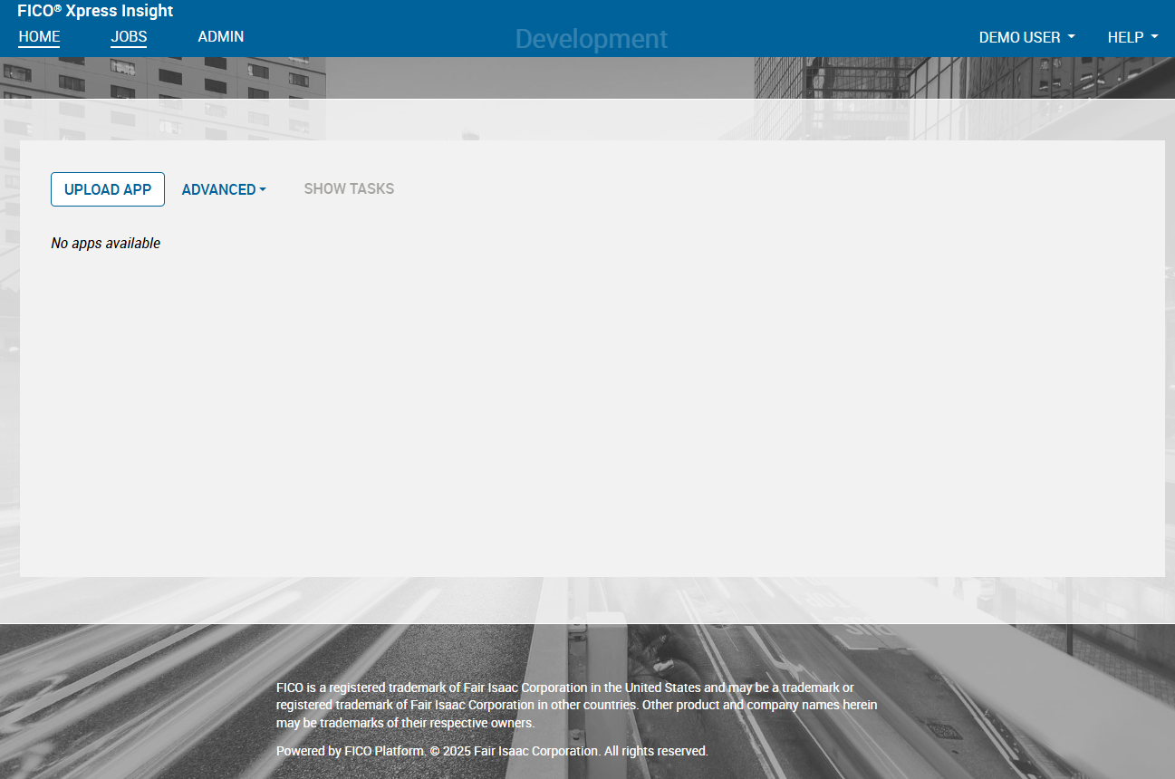
Figure 15.4: Xpress Insight web client entry page

If you have currently loaded any apps in Insight these will show up on the Web Client entry page, otherwise this page only displays the 'Upload app' icon. We now upload the app archive folioinsightxml.zip that adds a VDL view definition file and an XML configuration file to the archive folioinsight.zip. The Python model has been extended with a scalar entitiy to store the value of the total return after a solution has been obtained, a dataframe CtrSol to store data related to the constraints, and a CtrSummary series to display a summary of the result values for constraints in a convenient format for display (note the argument manage=xi.Manage.RESULT that is required to inform Xpress Insight that these entities are not input but result values).

Within the RUN mode function definition, after the execution of the optimization model, the solution values are now retrieved and stored in a new column of the Shares dataframe. Then, all the result entities are populated using the solution values:

@xi.AppConfig(name="Portfolio optimization", version=xi.AppVersion(1, 0, 0))
class InsightApp(xi.AppBase):

    ...

    # Result entities
    TotalReturn: xi.types.Scalar(dtype=xi.real, alias="Total expected return on investment",
        manage=xi.Manage.RESULT)

    CtrSolIds: xi.types.Index(dtype=xi.string, alias="Constraints", manage=xi.Manage.RESULT)
    CtrSol: xi.types.DataFrame(index="CtrSolIds", columns=[
        xi.types.Column("Activity", dtype=xi.real, alias="Activity", manage=xi.Manage.RESULT),
        xi.types.Column("LowerLimit", dtype=xi.real, alias="Lower limit",
            manage=xi.Manage.RESULT),
        xi.types.Column("UpperLimit", dtype=xi.real, alias="Upper limit",
            manage=xi.Manage.RESULT),
    ])


    CtrSumIds: xi.types.Index(dtype=xi.string, alias="Constraints", manage=xi.Manage.RESULT)
    CtrSummary: xi.types.Series(index="CtrSumIds", dtype=xi.real, manage=xi.Manage.RESULT)

    # Constant class attribute
    DATAFILE = "shares.csv"

    ...

    @xi.ExecModeRun(descr="Solve problem and initialize all result entities.")
    def run(self)

        ...

        # Solve optimization problem
        p.optimize()

        # Save results and key indicator values for GUI display
        self.Shares["fraction"] = pd.Series(p.getSolution(), index=self.ShareIds)
        self.TotalReturn = p.attributes.objval

        self.CtrSol = pd.DataFrame(columns=["Activity", "LowerLimit", "UpperLimit"])
        self.CtrSol.loc["Limit high risk shares"] = {
            "Activity": sum(self.Shares.loc[self.Shares.HighRisk, 'fraction']),
            "LowerLimit": 0,
            "UpperLimit": self.MaxHighRisk}

        self.CtrSol.loc["Limit North-American"] = {
            "Activity": sum(self.Shares.loc[self.Shares.NorthAmerica, 'fraction']),
            "LowerLimit": self.MinNorthAmerica,
            "UpperLimit": 1}

        for s in self.ShareIds:
            if self.Shares.loc[s, 'fraction'] > 0:
                self.CtrSol.loc[f"Limit per value: {s}"] = {
                    "Activity": self.Shares.loc[s, 'fraction'],
                    "LowerLimit": 0,
                    "UpperLimit": self.MaxPerShare}

        self.CtrSolIds = self.CtrSol.index

        self.CtrSummary = pd.Series()
        self.CtrSummary.loc["Largest position"] = max(self.Shares.fraction)
        self.CtrSummary.loc["Total high risk shares"] = \
            sum(self.Shares.loc[self.Shares.HighRisk, 'fraction'])
        self.CtrSummary.loc["Total North-American"] = \
            sum(self.Shares.loc[self.Shares.NorthAmerica, 'fraction'])
        self.CtrSummary.loc["Total return"] = p.attributes.objval

        self.CtrSumIds = self.CtrSummary.index

        print('Optimization finished.')

...

Once you have successfully loaded the app archive, the app 'Portfolio optimization' will show up as a new icon:

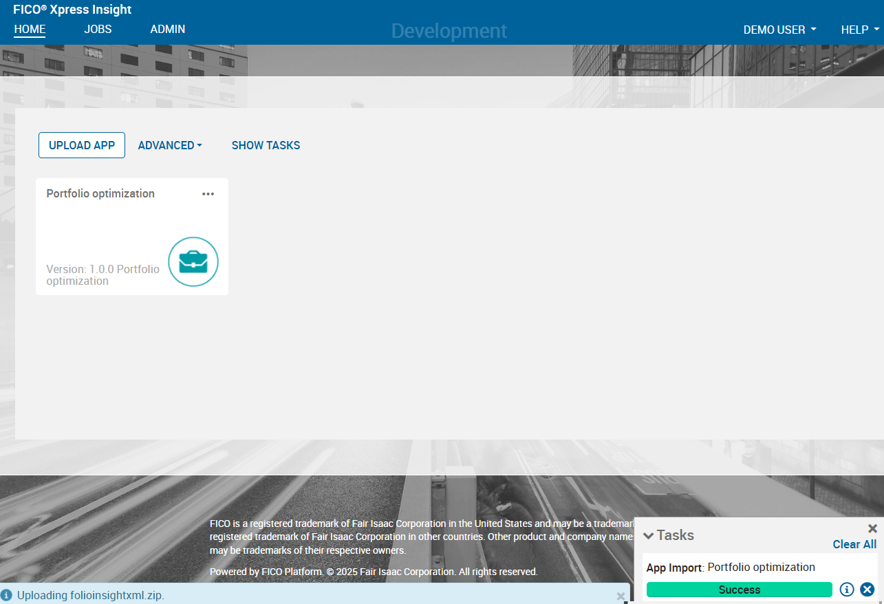
Figure 15.5: Xpress Insight web client after loading the Portfolio app

Select the 'Portfolio optimization' app icon to open the app. Note that if you have deployed an app from Workbench and followed the link 'Open in Xpress Insight' you will immediately be taken to this page.

Figure 15.6: App entry page

Now click on the text Open Scenario Manager in the shelf to create a scenario. In the 'Scenario Manager' window, double click 'Scenario 1' to put it on the shelf, then click CLOSE.

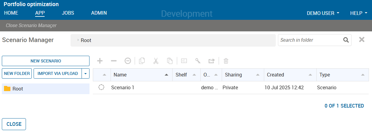
Figure 15.7: Scenario creation in the Xpress Insight web client

Use the Load entry from the drop-down menu on the scenario name in the shelf to load the baseline data.

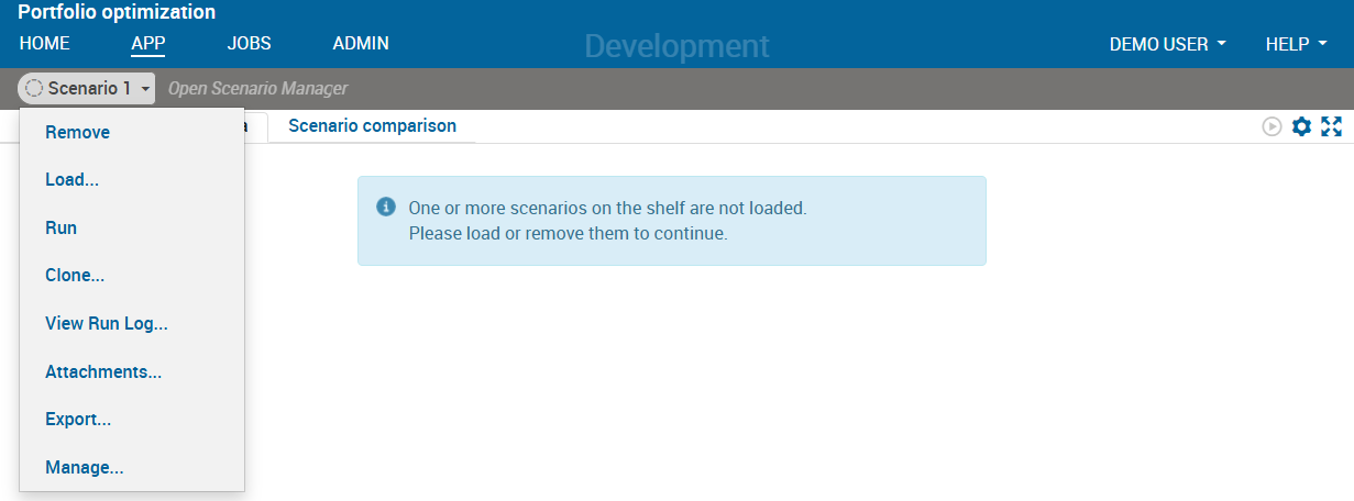
Figure 15.8: Scenario menu in the Xpress Insight web client

After loading the scenario the view display changes, showing the input data of our optimization model. You can edit these data by entering new values into the input fields or table cells. Use the Run button on the view or the corresponding entry in the scenario menu to run the model with the data shown on screen.

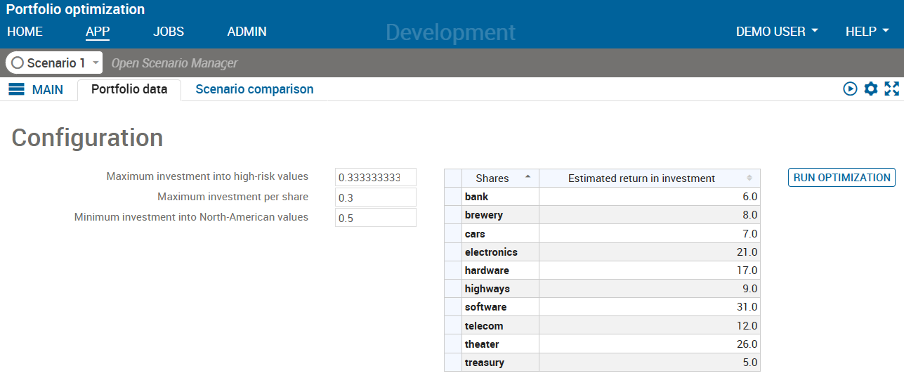
Figure 15.9: Display after scenario loading

After a successful model run the placeholder messages no data available in the lower half of our view are replaced by the results display, as shown below.

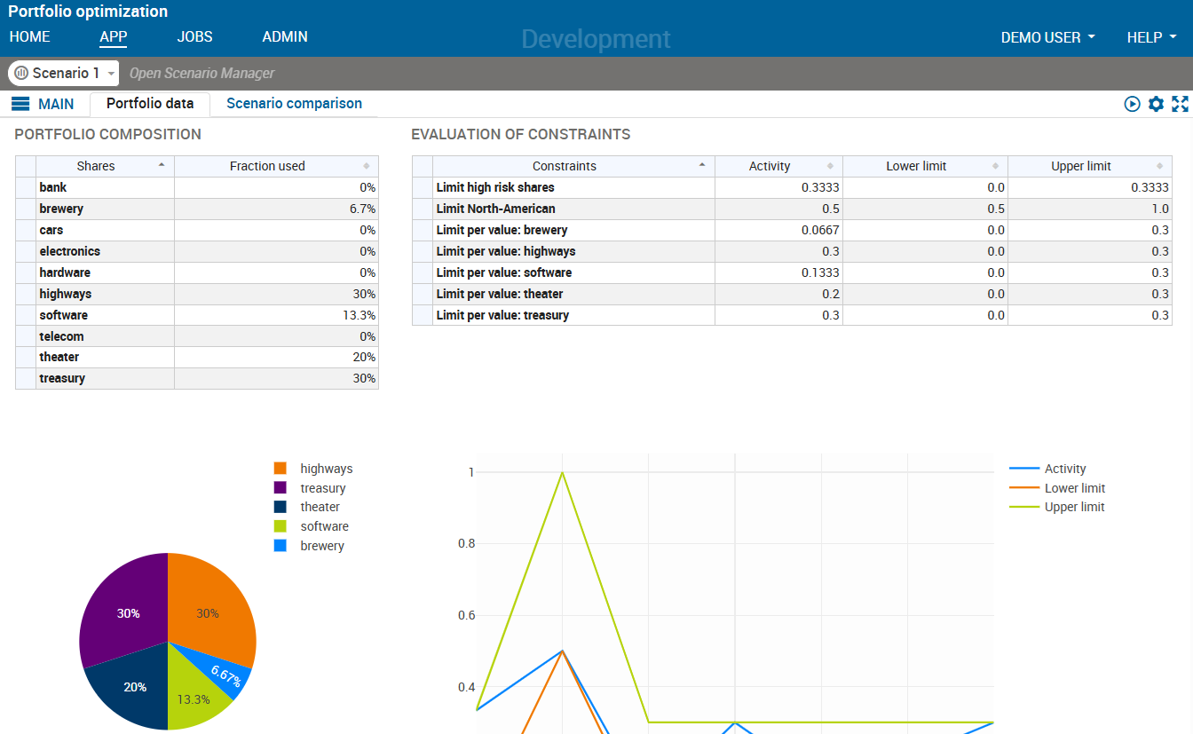
Figure 15.10: VDL view with input and result data elements

You can create new scenarios from existing ones (selecting 'Clone' in the scenario menu) or with the original input data by selecting 'New scenario' in the Scenario Explorer window. The results of multiple scenarios can be displayed in a single view for comparison.

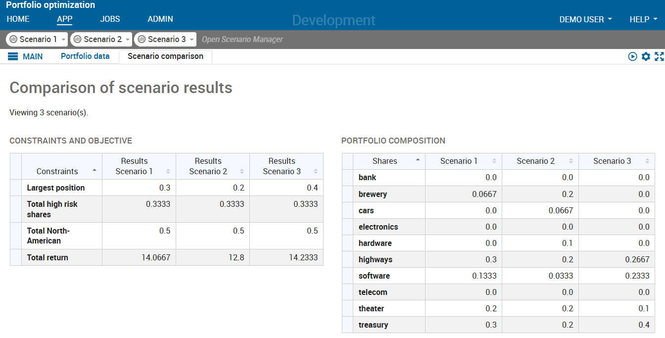
Figure 15.11: VDL view comparing several scenarios

VDL

VDL (View Definition Language) is a markup language for the creation of views for Xpress Insight apps from a set of predefined components and built-in styling options. Optionally, VDL view definitions can be extended with HTML tags and Javascript code for further customization.

Xpress Workbench includes a drag-and-drop editor for the creation and editing of VDL views. Within Xpress Workbench, select menu File » New » Insight View (VDL) to launch the view creation dialog. Enter 'Portfolio data' as the view title and folio.vdl as the filename for the view and in the following screen select 'Basic view' layout before terminating the dialog with 'Finish'. In the drag-and-drop editor that now shows, drag objects from the palette on the left onto the central artboard area—when doing so the editor will provide guidance regarding which combinations of objects are permitted (for example, a 'row' needs to contain 'columns' into which you can then add objects like 'table', 'chart' or 'text').

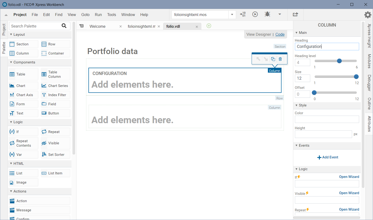
Figure 15.12: VDL view designer in Xpress Workbench

The attributes for the currently selected element in the editor can be edited in the pane on the right hand side.

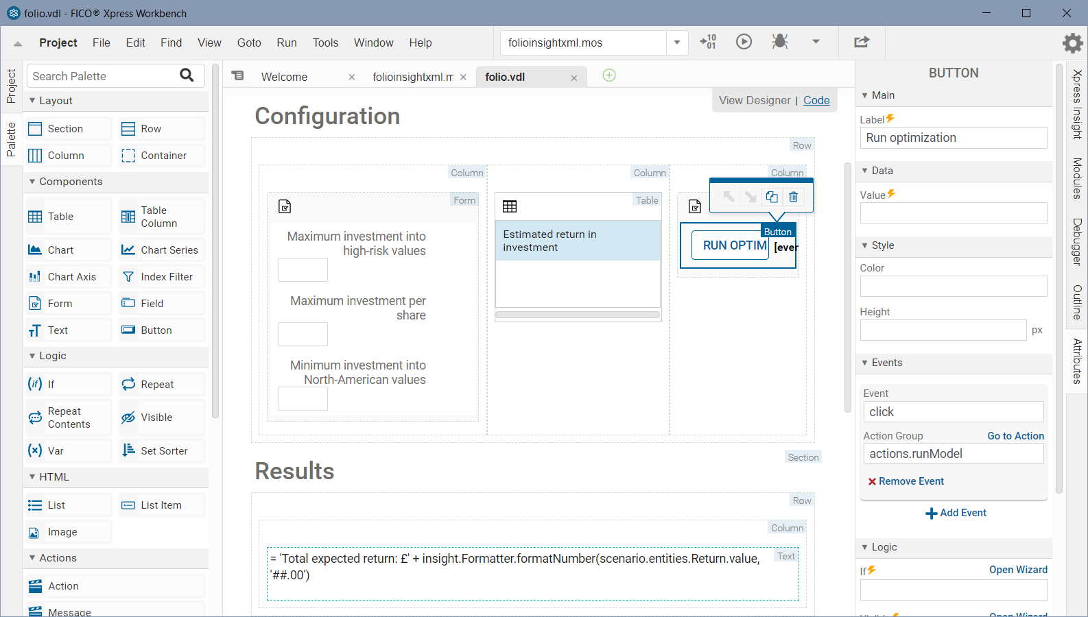
Figure 15.13: VDL view designer: editing view elements

For certain elements (table, chart) specific dialog windows will open to guide the user through their configuration.

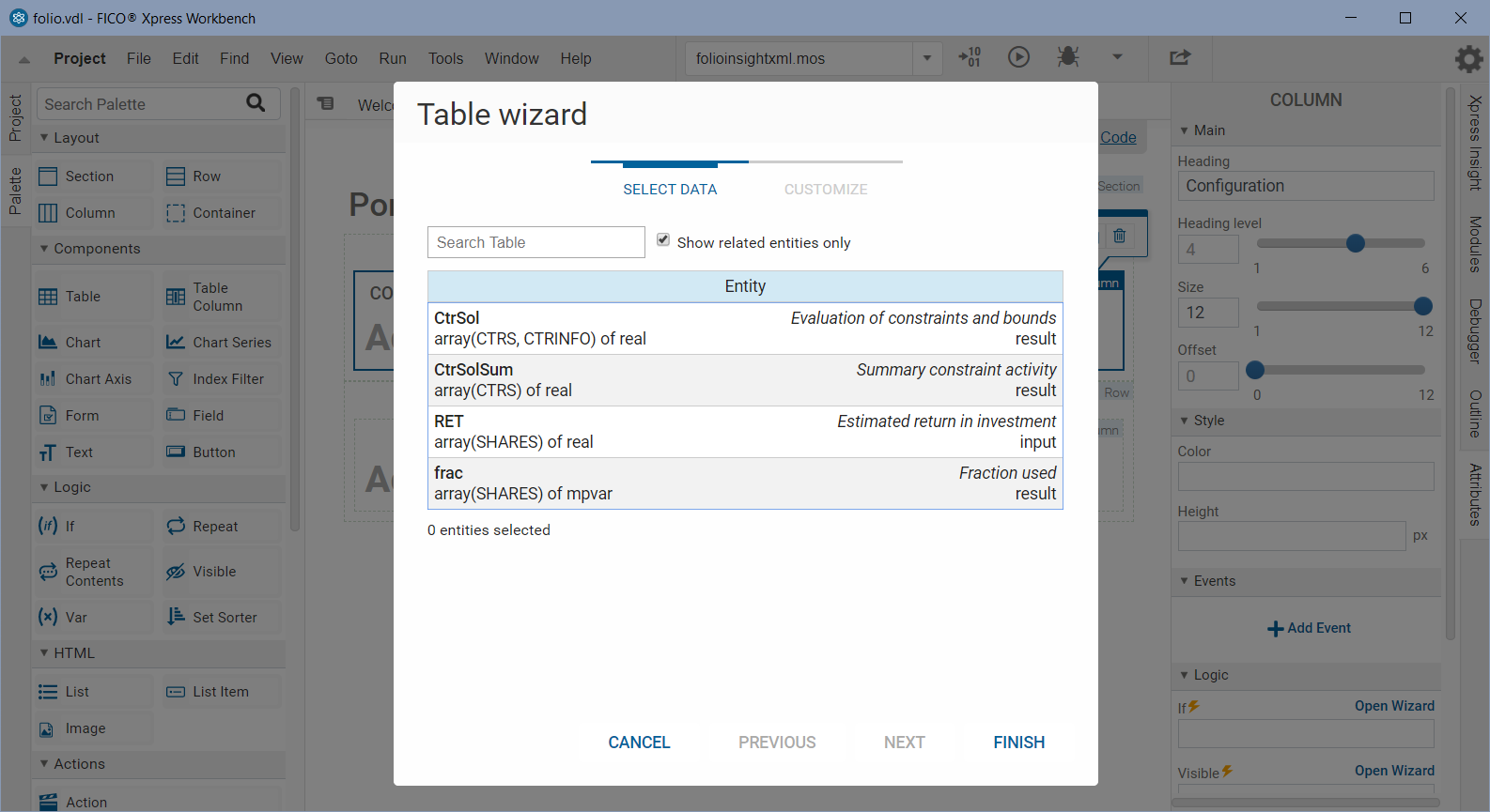
Figure 15.14: VDL view designer: table definition wizard

Note that at any time during the editing of VDL views in Workbench the app can be published to Insight by selecting the button in order to inspect the actual appearance of the web views when they are populated with scenario data.

The view 'Portfolio data' shown as web view in Figure VDL view with input and result data elements and in the VDL designer in Figure VDL view designer: editing view elements is created entirely from the following VDL view definition (file folio.vdl in the subdirectory client_resources of the app archive). All data entities marked as 'editable' can be modified by the UI user.

<vdl version="5">
  <vdl-page>
  <!-- 'vdl' and 'vdl-page' tags must always be present -->

    <!-- 'header' element: container for any vdl elements that are not part
         of the page layout -->
    <vdl-header>
        <vdl-action-group name="runModel">
          <vdl-action-execute mode="RUN"></vdl-action-execute>
        </vdl-action-group>
    </vdl-header>

    <!-- Structural element 'section': print header text for a section -->
    <vdl-section heading="Configuration">

      <!-- Structural element 'row': arrange contents in rows -->
      <vdl-row>
        <!-- Several columns within a 'row' for display side-by-side,
             dividing up the total row width of 12 via 'size' setting
             on each column. -->
        <vdl-column size="5">
          <!-- A form groups several input elements -->
          <vdl-form>
            <!-- Input fields for constraint limits -->
            <vdl-field parameter="MaxHighRisk" size="3" label-size="9"
              label="Maximum investment into high-risk values"/>
            <vdl-field parameter="MaxPerShare" size="3" label-size="9"
              label=" Maximum investment per share"/>
            <vdl-field parameter="MinNorthAmerica" size="3" label-size="9"
              label="Minimum investment into North-American values" />
            <!-- default sizes: 2 units each -->
          </vdl-form>
        </vdl-column>
        <vdl-column size="4">
          <!-- Display editable input values, default table format -->
          <vdl-table>
            <vdl-table-column entity="Shares_Return" editable="true"/>
          </autotable>
        </vdl-column>
        <vdl-column size="3">
          <vdl-form>
            <!-- 'Run' button to launch optimization -->
            <vdl-button vdl-event="click:actions.runModel"
              label="Run optimization"></vdl-button>
          </vdl-form>
        </vdl-column>
      </vdl-row>
    </vdl-section>


    <!-- Placeholder message for 'Results' section -->
    <vdl-container vdl-if="=!scenario.summaryData.hasResultData">
      <span vdl-text="no results available"></span></vdl-container>

    <!-- Structural element 'section';
         display: with option 'none' nothing gets displayed by default
         if hasResultData: display section once result values become available
                           (after scenario execution) -->
    <vdl-section heading="Results"
         vdl-if="=scenario.summaryData.hasResultData" style="display: none">

      <vdl-row>
        <vdl-column>
          <!-- Display text element with the objective value -->
          <span vdl-text="='Total expected return: &#163;' +
              insight.Formatter.formatNumber(scenario.entities.TotalReturn.value,
              '##.00')"></span>
      </vdl-row>

      <vdl-row>
        <vdl-column size="4" heading="Portfolio composition">
          <!-- Display the 'fraction' solution values, default table format -->
          <vdl-table>
            <vdl-table-column entity="Shares_fraction" render="=formatRender">
            </vdl-table-column>
          </vdl-table>
        </vdl-column>
        <vdl-column size="8">
          <!-- Display the 'frac' solution values as a pie chart -->
          <vdl-chart style="width:400px;">
            <vdl-chart-series entity="Shares_fraction" type="pie"></vdl-chart-series>
          </vdl-chart>
        </vdl-column>
      </vdl-row>
    </vdl-section>
  </vdl-page>
</vdl> 

VDL views need to be declared in an app archive via an XML configuration file (the so-called companion file). When VDL views are created via the view designer in Workbench then the required entry is added automatically to this file. Companion files can also be created and edited using the Workbench editor (select File » New » Companion file ). The following companion file definition integrates the VDL view folio.vdl and a second view 'Scenario comparison' into our example app folioinsightxml.zip.

<?xml version="1.0" encoding="UTF-8"?>
<model-companion xmlns="http://www.fico.com/xpress/optimization-modeler/model-companion"
    version="5.0">
  <client>
    <view-group title="Main">
      <vdl-view title="Portfolio data" path="folio.vdl" />
      <vdl-view title="Scenario comparison" default="false" path="foliocompare.vdl" />
    </view-group>
  </client>
</model-companion>