Solution Methods

Topics covered in this chapter:

The FICO Xpress Optimization Suite provides four fundamental optimization algorithms for LP or QP problems: the primal simplex, the dual simplex, the hybrid gradient and the Newton barrier algorithm (QCQP and SOCP problems are always solved with the Newton barrier algorithm). Using these algorithms the Optimizer implements solving functionality for the various types of continuous problems the user may want to solve.

Typically the user will allow the Optimizer to choose what combination of methods to use for solving their problem. For example, by default, the FICO Xpress Optimizer uses the dual simplex method for solving LP problems and the barrier method for solving QP problems. For the initial continuous relaxation of a MIP, the defaults will be different and depends both on the number of solver threads used, the type of the problem and the MIP technique selected.

For most users the default behavior of the Optimizer will provide satisfactory solution performance and they need not consider any customization. However, if a problem seems to be taking an unusually long time to solve or if the solving performance is critical for the application, the user may consider, as a first attempt, to force the Optimizer to use an algorithm other than the default.

The main points where the user has a choice of what algorithm to use are (i) when the user calls the optimization routine XPRSlpoptimize (LPOPTIMIZE) and (ii) when the Optimizer solves the node relaxation problems during the branch and bound search. The user may force the use of a particular algorithm by specifying flags to the optimization routine XPRSlpoptimize (LPOPTIMIZE). If the user specifies flags to XPRSmipoptimize (MIPOPTIMIZE) to select a particular algorithm then this algorithm will be used for the initial relaxation only. To specify what algorithm to use when solving the node relaxation problems during branch and bound use the special control parameter, DEFAULTALG.

As a guide for choosing optimization algorithms other than the default consider the following. As a general rule, the dual simplex is usually much faster than the primal simplex if the problem is neither infeasible nor near-infeasible. If the problem is likely to be infeasible or if the user wishes to get diagnostic information about an infeasible problem then the primal simplex is the best choice. This is because the primal simplex algorithm finds a basic solution that minimizes the sum of infeasibilities and these solutions are typically helpful in identifying causes of infeasibility. The Newton barrier algorithm can perform much better than the simplex algorithms on certain classes of problems. The barrier algorithm will, however, likely be slower than the simplex algorithms if, for a problem coefficient matrix A, A^TA is large and dense.

The hybrid gradient algorithm can be used only for LP problems. It is especially useful on very degenerate problems, and, thanks to its low memory usage, on extremely large problems.

In the following few sections, performance issues relating to these methods will be discussed in more detail. Performance issues relating to the search for MIP solutions will also be discussed.

Simplex Method

The simplex method was the first efficient method devised for solving Linear Programs (LPs). This method is still commonly used today and there are efficient implementations of the primal and dual simplex methods available in the Optimizer. We briefly outline some basic simplex theory to give the user a general idea of the simplex algorithm's behavior and to define some terminology that is used in the reference sections.

A region defined by a set of constraints is known in Mathematical Programming as a feasible region. When these constraints are linear the feasible region defines the solution space of a Linear Programming (LP) problem. Each value of the objective function of an LP defines a hyperplane or a level set. A fundamental result of simplex algorithm theory is that an optimal value of the LP objective function will occur when the level set grazes the boundary of the feasible region. The optimal level set either intersects a single point (or vertex) of the feasible region (if such a point exists), in which case the solution is unique, or it intersects a boundary set of the feasible region in which case there is an infinite set of solutions.

In general, vertices occur at points where as many constraints and variable bounds as there are variables in the problem intersect. Simplex methods usually only consider solutions at vertices, or bases (known as basic solutions) and proceed or iterate from one vertex to another until an optimal solution has been found, or the problem proves to be infeasible or unbounded. The number of iterations required increases with model size, and typically goes up slightly faster than the increase in the number of constraints.

The primal and dual simplex methods differ in which vertices they consider and how they iterate. The dual is the default for LP problems, but may be explicitly invoked using the d flag with XPRSlpoptimize (LPOPTIMIZE).

Output

While the simplex methods iterate, the Optimizer produces iteration logs. The Console Optimizer writes these logging messages to the screen. Library users can setup logging management using the various relevant functions in the Optimizer library e.g., XPRSsetlogfile, XPRSaddcbmessage or XPRSaddcblplog. The simplex iteration log is produced at regular time intervals, determined by an internal deterministic. When LPLOG is set to 0, a log is displayed only when the optimization run terminates. If it is set to a positive value, a summary style log is output; otherwise, a detailed log is output.

Newton Barrier Method

In contrast to the simplex methods that iterate through boundary points (vertices) of the feasible region, the Newton barrier method iterates through solutions in the interior of the feasible region and will typically find a close approximation of an optimal solution. Consequently, the number of barrier iterations required to complete the method on a problem is determined more so by the required proximity to the optimal solution than the number of decision variables in the problem. Unlike the simplex method, therefore, the barrier often completes in a similar number of iterations regardless of the problem size.

The barrier solver can be invoked on a problem by using the 'b' flag with XPRSlpoptimize (LPOPTIMIZE). This is used by default for QP problems, whose quadratic objective functions in general result in optimal solutions that lie on a face of the feasible region, rather than at a vertex.

Crossover

Typically the barrier algorithm terminates when it is within a given tolerance of an optimal solution. Since this solution will not lie exactly on the boundary of the feasible region, the Optimizer can be optionally made to perform a, so-called, 'crossover' phase to obtain an optimal solution on the boundary. The nature of the 'crossover' phase results in a basic optimal solution, which is at a vertex of the feasible region. In the crossover phase the simplex method is used to continue the optimization from the solution found by the barrier algorithm. The CROSSOVER control determines whether the Optimizer performs crossover. When set to 1 (the default for LP problems), crossover is performed. If CROSSOVER is set to 0, no crossover will be attempted and the solution provided will be that determined purely by the barrier method. Note that if a basic optimal solution is required, then the CROSSOVER option must be activated before optimization starts.

Output

While the barrier method iterates, the Optimizer produces iteration log messages. The Console Optimizer writes these log messages to the screen. Library users can setup logging management using the various relevant functions in the Optimizer library, e.g. XPRSsetlogfile, XPRSaddcbmessage or XPRSaddcbbarlog. Note that the amount of barrier iteration logging is dependent on the value of the BAROUTPUT control.

Hybrid Gradient Method

Similar to the Newton barrier algorithm, the hybrid gradient method iterates through solutions in the interior of the feasible region and will typically find a close approximation of an optimal solution. The number of hybrid gradient iterations required to complete the method is typically large, but each iteration is very fast.

The hybrid gradient solver can be invoked on a problem by using the 'b' flag with XPRSlpoptimize (LPOPTIMIZE) and setting BARALG to 4.

The hybrid gradient method is the implementation of a first-order primal-dual alternating directions method. As such, its rate of convergence is only linear, thus it is not designed to achieve the accuracy of some of the other algorithms, most notably that of the Newton barrier methods. For this reason it is advised to relax the feasibility (BARPRIMALSTOP) and optimality tolerances (BARDUALSTOP). By default they are 100 times the defaults we would have in the Newton barrier algorithm.

Crossover

The hybrid gradient algorithm terminates when the solution it has found is within a given tolerance of an optimal solution. This solution is typically not on the boundary of the feasible set. A crossover phase, similar to the one applied after the Newton barrier method, can be used to arrive at a basic solution.

Output

The format and content of the hybrid gradient method log is identical to the Newton barrier log with a few notable differences: since no Cholesky decomposition is performed the table about matrix density is not printed. Also, upper bound infeasibility is always 0.

Branch and Bound

The FICO Xpress Optimizer uses the approach of LP based branch and bound with cutting planes for solving Mixed Integer Programming (MIP) problems. That is, the Optimizer solves the optimization problem (typically an LP problem) resulting from relaxing the discreteness constraints on the variables and then uses branch and bound to search the relaxation space for MIP solutions. It combines this with heuristic methods to quickly find good solutions, and cutting planes to strengthen the LP relaxations.

The Optimizer's MIP solving methods are coordinated internally by sophisticated algorithms so the Optimizer will work well on a wide range of MIP problems with a wide range of solution performance requirements without any user intervention in the solving process. Despite this the user should note that the formulation of a MIP problem is typically not unique and the solving performance can be highly dependent on the formulation of the problem. It is recommended, therefore, that the user undertake careful experimentation with the problem formulation using realistic examples before committing the formulation for use on large production problems. It is also recommended that users have small scale examples available to use during development.

Because of the inherent difficulty in solving MIP problems and the variety of requirements users have on the solution performance on these problems it is not uncommon that users would like to improve over the default performance of the Optimizer. In the following sections we discuss aspects of the branch and bound method for which the user may want to investigate when customizing the Optimizer's MIP search.

Theory

In this section we present a brief overview of branch and bound theory as a guide for the user on where to look to begin customizing the Optimizer's MIP search and also to define the terminology used when describing branch and bound methods.

To simplify the text in the following, we limit the discussion to MIP problems with linear constraints and a linear objective function. Note that it is not difficult to generalize the discussion to problems with quadratic constraints and a quadratic objective function.

The branch and bound method has three main concepts: relaxation, branching and fathoming.

The relaxation concept relates to the way discreteness or integrality constraints are dropped or 'relaxed' in the problem. The initial relaxation problem is a Linear Programming (LP) problem which we solve resulting in one of the following cases:

1. The LP is infeasible so the MIP problem must also be infeasible;
2. The LP has a feasible solution, but some of the integrality constraints are not satisfied – the MIP has not yet been solved;
3. The LP has a feasible solution and all the integrality constraints are satisfied so the MIP has also been solved;
4. The LP is unbounded.

Case (d) is a special case. It can only occur when solving the initial relaxation problem and in this situation the MIP problem itself is not well posed (see Chapter Infeasibility, Unboundedness and Instability for details about what to do in this case). For the remaining discussion we assume that the LP is not unbounded.

Outcomes (a) and (c) are said to 'fathom' the particular MIP, since no further work on it is necessary. For case (b) more work is required, since one of the unsatisfied integrality constraints must be selected and the concept of separation applied.

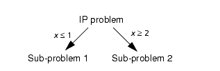
To illustrate the branching concept suppose, for example, that the optimal LP value of an integer variable x is 1.34, a value which violates the integrality constraint. It follows that in any solution to the original problem either x ≤ 1.0 or x ≥2.0. If the two resulting MIP problems are solved (with the integrality constraints), all integer values of x are considered in the combined solution spaces of the two MIP problems and no solution to one of the MIP problems is a solution to the other. In this way we have branched the problem into two disjoint sub-problems.

If both of these sub-problems can be solved and the better of the two is chosen, then the MIP is solved. By recursively applying this same strategy to solve each of the sub-problems and given that in the limiting case the integer variables will have their domains divided into fixed integer values then we can guarantee that we solve the MIP problem.

Branch and bound can be viewed as a tree search algorithm. Each node of the tree is a MIP problem. A MIP node is relaxed and the LP relaxation is solved. If the LP relaxation is not fathomed, then the node MIP problem is partitioned into two more sub-problems, or child nodes. Each child MIP will have the same constraints as the parent node MIP, plus one additional inequality constraint. Each node is therefore either fathomed or has two children or descendants.

We now introduce the concept of a cutoff, which is an extension of the fathoming concept. To understand the cutoff concept we first make two observations about the behavior of the node MIP problems. Firstly, the optimal MIP objective of a node problem can be no better than the optimal objective of the LP relaxation. Secondly, the optimal objective of a child LP relaxation can be no better than the optimal objective of its parent LP relaxation. Now assume that we are exploring the tree and we are keeping the value of the best MIP objective found so far. Assume also that we keep a 'cutoff value' equal to the best MIP objective found so far. To use the cutoff value we reason that if the optimal LP relaxation objective is no better than the cutoff then any MIP solution of a descendant can be no better than the cutoff and the node can be fathomed (or cutoff) and need not be considered further in the search.

The concept of a cutoff can be extended to apply even when no integer solution has been found in situations where it is known, or may be assumed, from the outset that the optimal solution must be better than some value. If the relaxation is worse than this cutoff, then the node may be fathomed. In this way the user can reduce the number of nodes processed and improve the solution performance. Note that there is the possibility, however, that all MIP solutions, including the optimal one, may be missed if an overly optimistic cutoff value is chosen.

The cutoff concept may also be extended in a different way if the user intends only to find a solution within a certain tolerance of the overall optimal MIP solution. Assume that we have found a MIP solution to our problem and assume that the cutoff is maintained at a value 100 objective units better than the current best MIP solution. Proceeding in this way we are guaranteed to find a MIP solution within 100 units of the overall MIP optimal since we only cutoff nodes with LP relaxation solutions worse than 100 units better than the best MIP solution that we find.

If the MIP problem contains SOS entities then the nodes of the branch and bound tree are determined by branching on the sets. Note that each member of the set has a double precision reference row entry and the sets are ordered by these reference row entries. Branching on the sets is done by choosing a position in the ordering of the set variables and setting all members of the set to 0 either above or below the chosen point. The optimizer used the reference row entries to decide on the branching position and so it is important to choose the reference row entries which reflect the cost of setting the set member to 0. In some cases it maybe better to model the problem with binary variables instead of special ordered sets. This is especially the case if the sets are small.

Variable Selection and Cutting

The branch and bound technique leaves many choices open to the user. In practice, the success of the technique is highly dependent on several key choices.

1. Deciding which variable to branch on is known as the variable selection problem and is often the most critical choice.
2. Cutting planes are used to strengthen the LP relaxation of a subproblem, and can often bring a significant reduction in the number of sub-problems that must be solved

The Optimizer incorporates a default strategy for both choices which has been found to work adequately on most problems. Several controls are provided to tailor the search strategy to a particular problem.

Variable Selection for Branching

Each MIP entity has a priority for branching, or one set by the user in the directives file. A low priority value means that the variable is more likely to be selected for branching. The Optimizer uses a priority range of 400–500 by default. To guarantee that a particular MIP entity is always branched first, the user should assign a priority value less than 400. Likewise, to guarantee that a MIP entity is only branched on when it is the only candidate left, a priority value above 500 should be used.

The Optimizer uses a wide variety of information to select among those entities that remain unsatisifed and which belong to the lowest valued priority class. A pseudo cost is calculated for each candidate entity, which is typically an estimate of how much the LP relaxation objective value will change (degradationas a result of branching on this particular candidate. Estimates are calculated separately for the up and down branches and combined according to the strategy selected by the VARSELECTION control.

The default strategy is based on calculating pseudo costs using the method of strong branching. With strong brancing, the LP relaxations of the two potential subproblems that would result from branching on a candidate MIP entity, are solved partially. Dual simplex is applied for a limited number of iterations and the change in objective value is recorded as a pseudo cost. This can be very expensive to apply to every candidate for every node of the branch and bound search, which is why the Optimizer by default will reuse pseudo costs collected from one node, on subsequent nodes of the search.

Selecting a MIP entity for branching is a multi-stage process, which combines estimates that are cheap to compute, with the more expensive strong branching based pseudo costs. The basic selection process is given by the following outline, together with the controls that affect each step:

1. Pre-filter the set of candidate entities using very cheap estimates.
   SBSELECT: determine the filter size.
2. Calculate simple estimates based on local node information and rank the selected candidates.
   SBESTIMATE: local ranking function.
3. Calculate strong branching pseudo costs for candidates lacking such information.
   SBBEST: number of variables to strong branch on.
   SBITERLIMIT: LP iteration limit for strong branching.
4. Select the best candidate using a combination of pseudo costs and the local ranking functions.

The overall amount of effort put into this process can be adjusted using the SBEFFORT control.

Cutting Planes

Cutting planes are valid constraints used for tightening the LP relaxation of a MIP problem, without affecting the MIP solution space. They can be very effective at reducing the amount of subproblems that the branch and bound search has to solve. The Optimizer will automatically create many different well-known classes of cutting planes, such as mixed integer Gomory cuts, lift-and-project cuts, mixed integer rounding (MIR) cuts, clique cuts, implied bound cuts, flow-path cuts, zero-half cuts, etc. These classes of cuts are grouped together into two groups that can be controlled separately. The following table lists the main controls and the related cut classes that are affected by those control:

COVERCUTS	Mixed integer rounding cuts
TREECOVERCUTS	Lifted cover cuts
	Clique cuts
	Implied bound cuts
	Flow-path cuts
	Zero-half cuts
GOMCUTS	Mixed integer Gomory cuts
TREEGOMCUTS	Lift-and-project cuts

The controls COVERCUTS and GOMCUTS sets an upper limit on the number of rounds of cuts to create for the root problem, for their respective groups. Correspondingly, TREECOVERCUTS and TREEGOMCUTS sets an upper limit on the number of rounds of cuts for any subproblem in the tree.

An important aspect of cutting is the choice of how many cuts to add to a subproblem. The more cuts are added, the harder it becomes to solve the LP relaxation of the node problem. The tradeoff is therefore between the additional effort in solving the LP relaxation versus the strengthening of the subproblem. The CUTSTRATEGY control sets the general level of how many cuts to add, expressed as a value from 0 (no cutting at all) to 3 (high level of cuts).

Another important aspect of cutting is how often cuts should be created and added to a subproblem. The Optimizer will automatically decide on a frequency that attempts to balance the effort of creating cuts versus the benefits they provide. It is possible to override this and set a fixed strategy using the CUTFREQ control. When set to a value k, cutting will be applied to every k'th level of the branch and bound tree. Note that setting CUTFREQ = 0 will disable cutting on subproblems completely, leaving only cutting on the root problem. This might be advantageous for some problems and the Optimizer uses an ML-based strategy to detect such cases automatically. This feature can be (de)activated by the AUTOCUTTING control.

Node Selection

The Optimizer applies a search scheme involving best-bound first search combined with dives. Subproblems that have not been fathomed or which have not been branched further into new subproblems are referred to as active nodes of the branch and bound search tree. Such activate nodes are maintained by the Optimizer in a pool.

The search process involves selecting a subproblem (or node) from this active nodes pool and commencing a dive. When the Optimizer branches on a MIP entity and creates the two subproblems, it has a choice of which of the two subproblems to work on next. This choice is determined by the BRANCHCHOICE control. The dive is a recursive search, where it selects a child problem, branches on it to create two new child problems, and repeats with one of the new child problems, until it ends with a subproblem that should not be branched further. At this point it will go back to the active nodes pool and pick a new subproblem to perform a dive on. This is called a backtrack and the choice of node is determined by the BACKTRACK control. The default backtrack strategy will select the active node with the best bound.

Adjusting the Cutoff Value

The parameter MIPADDCUTOFF determines the cutoff value set by the Optimizer when it has identified a new MIP solution. The new cutoff value is set as the objective function value of the MIP solution plus the value of MIPADDCUTOFF. If MIPADDCUTOFF has not been set by the user, the value used by the Optimizer will be calculated after the initial LP optimization step as:

max (MIPADDCUTOFF, 0.01·MIPRELCUTOFF·LP_value)

using the initial values for MIPADDCUTOFF and MIPRELCUTOFF, and where LP_value is the optimal objective value of the initial LP relaxation.

Stopping Criteria

Often when solving a MIP problem it is sufficient to stop with a good solution instead of waiting for a potentially long solve process to find an optimal solution. The Optimizer provides several stopping criteria related to the solutions found, through the MIPRELSTOP and MIPABSSTOP parameters. If MIPABSSTOP is set for a minimization problem, the Optimizer will stop when it finds a MIP solution with an objective value equal to or less than MIPABSSTOP. The MIPRELSTOP parameter can be used to stop the solve process when the found solution is sufficiently close to optimality, as measure relative to the best available bound. The optimizer will stop due to MIPRELSTOP when the following is satisfied:

| MIPOBJVAL – BESTBOUND | ≤ MIPRELSTOP · max( | BESTBOUND |, | MIPOBJVAL | )

It is also possible to set limits on the solve process, such as number of nodes (MAXNODE), time limit (MAXTIME) or on the number of solutions found (MAXMIPSOL). If the solve process is interrupted due to any of these limits, the problem will be left in its unfinished state. It is possible to resume the solve from an unfinished state by calling XPRSmipoptimize (MIPOPTIMIZE) again.

To return an unfinished problem to its starting state, where it can be modified again, the user should use the function XPRSpostsolve (POSTSOLVE). This function can be used to restore a problem from an interrupted tree search even if the problem is not in a presolved state.

Integer Preprocessing

If MIPPRESOLVE has been set to a nonzero value before solving a MIP problem, integer preprocessing will be performed at each node of the branch and bound tree search (including the root node). This incorporates reduced cost tightening of bounds and tightening of implied variable bounds after branching. If a variable is fixed at a node, it remains fixed at all its child nodes, but it is not deleted from the matrix (unlike the variables fixed by presolve).

MIPPRESOLVE is a bitmap whose values are acted on as follows:

Bit	Value	Action
0	1	Reduced cost fixing;
1	2	Integer implication tightening.
2	4	Unused
3	8	Tightening of implied continuous variables.
4	16	Fixing of variables based on dual (i.e. optimality) implications.

So a value of 1+2=3 for MIPPRESOLVE causes reduced cost fixing and tightening of implied bounds on integer variables.

Convex QCQP and SOCP Methods

Convex continuous QCQP and SOCP problems are solved by the Xpress Newton-barrier solver. For QCQP, SOCP and QP problems, there is no solution purification method applied after the barrier (such as the crossover for linear problems). This means that solutions tend to contain more active variables than basic solutions, and fewer variables will be at or close to one of their bounds.

When solving a linearly constrained quadratic program (QP) from scratch, the Newton barrier method is usually the algorithm of choice. In general, the quadratic simplex methods are better if a solution with a low number of active variables is required, or when a good starting basis is available (e.g., when reoptimizing).

Non-convex QCQP problems are solved by a branch-and-bound approach, see the FICO Xpress Global userguide for more details.

Convexity Checking

Problems with quadratic constraints or quadratic objective are automatically checked for convexity to determine whether the global solver is needed. The Newton-barrier and quadratic simplex solvers require that the quadratic coefficient matrix in each constraint or in the objective function is either positive semi-definite or negative semi-definite, depending on the sense of for constraints or the direction of optimization for the objective. The only exception is when a quadratic constraint describes a second order cone. Note that the convexity checker will reject any problem where this requirement is violated by more than a small tolerance.

Each constraint is checked individually for convexity. In certain cases it is possible that the problem itself is convex, but the representation of it is not. A simple example would be

minimize:	x
subject to:	x2–y2+2xy	≤	1
	y=0

The global solver will be selected to solve this problem if the automatic convexity check is on, although the problem is clearly convex. The reason is that convexity of QCQPs is checked before any presolve takes place. To understand why, consider the following example:

minimize:	y
subject to:	y–x2	≤	1
	y=2

This problem is clearly feasible, and an optimal solution is (x,y)=(1,2). However, when presolving the problem, it will be found infeasible, since assuming that the quadratic part of the first constraint is convex the constraint cannot be satisfied (remember that if a constraint is convex, then removing the quadratic part is always a relaxation). Thus since presolve makes use of the assumption that the problem is convex, convexity must be checked before presolve.

Note that for quadratic programming (QP) and mixed integer quadratic programs (MIQP) where the quadratic expressions appear only in the objective, the convexity check takes place after presolve, making it possible to accept matrices that are not PSD, but define a convex function over the feasible region (note that this is only a chance).

Quadratically Constrained and Second Order Cone Problems

Quadratically constrained and second order cone problems are solved by the barrier algorithm.

Mixed integer quadratically constrained (MIQCQP) and mixed integer second order problems (MISOCP) are solved using traditional branch and bound using the barrier to solve the node problems, or by means of outer approximation, as defined by control MIQCPALG.

It is sometimes beneficial to solve the root node of an MIQCQP or MISOCP by the barrier, even if outer approximation is used later; controlled by the QCROOTALG control. The number of cut rounds on the root for outer approximation is defined by QCCUTS.