
Scheduling
Topics covered in this chapter:
- Tasks and resources
- Precedences
- Disjunctive scheduling: unary resources
- Cumulative scheduling: discrete resources
- Renewable and non-renewable resources
- Extensions: setup times, resource choice, usage profiles
- Enumeration
This chapter shows how to
- define and setup the modeling objects cptask and cpresource,
- formulate and solve scheduling problems using these objects,
- access information from the modeling objects.
- parameterize search strategies involving the scheduling objects,
Tasks and resources
Scheduling and planning problems are concerned with determining a plan for the execution of a given set of tasks. The objective may be to generate a feasible schedule that satisfies the given constraints (such as sequence of tasks or limited resource availability) or to optimize a given criterion such as the makespan of the schedule.
Xpress Kalis defines several aggregate modeling objects to simplify the formulation of standard scheduling problems: tasks (processing operations, activities) are represented in Mosel by the type cptask and resources (machines, raw material etc.) by the type cpresource. When working with these scheduling objects it is often sufficient to state the objects and their properties, such as task duration or resource use; the necessary constraint relations are set up automatically by Xpress Kalis (referred to as implicit constraints). In the following sections we show a number of examples using this mechanism:
- The simplest case of a scheduling problem involves only tasks and precedence constraints between tasks (project scheduling problem in Section Precedences).
- Tasks may be mutually exclusive, e.g. because they use the same unitary resource (disjunctive scheduling / sequencing problem in Section Disjunctive scheduling: unary resources).
- Resources may be usable by several tasks at a time, up to a given capacity limit (cumulative resources, see Section Cumulative scheduling: discrete resources).
- A different classification of resources is the distinction between renewable and non-renewable resources (see Section Renewable and non-renewable resources).
- Many extensions of the standard problems are possible, such as sequence-dependent setup time (see Section Setup times), choice of resources (Section Alternative resources), tasks with non-constant resource profiles (Section Resource profiles), or given idle times for resources (Section Resource idle times and preemption of tasks).
If the enumeration is started with the function cp_schedule the solver will employ specialized search strategies suitable for the corresponding (scheduling) problem type. It is possible to parameterize these strategies or to define user search strategies for scheduling objects (see Section Enumeration). Alternatively, the standard optimization functions cp_minimize / cp_maximize may be used. In this case the enumeration does not exploit the structural information provided by the scheduling objects and works simply with decision variables.
The properties of scheduling objects (such as start time or duration of tasks) can be accessed and employed, for instance, in the definition of constraints, thus giving the user the possibility to extend the predefined standard problems with other types of constraints. For even greater flexibility Xpress Kalis also enables the user to formulate his scheduling problems without the aggregate modeling objects, using dedicated global constraints on decision variables of type cpvar. Most examples in this chapter are therefore given with two different implementations, one using the scheduling objects and another without these objects.
Precedences
Probably the most basic type of a scheduling problem is to plan a set of tasks that are linked by precedence constraints.
The problem described in this section is taken from Section 7.1 `Construction of a stadium' of the book `Applications of optimization with Xpress-MP'
A construction company has been awarded a contract to construct a stadium and wishes to complete it within the shortest possible time. Table Data for stadium construction lists the major tasks and their durations in weeks. Some tasks can only start after the completion of certain other tasks, equally indicated in the table.
| Task | Description | Duration | Predecessors |
|---|---|---|---|
| 1 | Installing the construction site | 2 | none |
| 2 | Terracing | 16 | 1 |
| 3 | Constructing the foundations | 9 | 2 |
| 4 | Access roads and other networks | 8 | 2 |
| 5 | Erecting the basement | 10 | 3 |
| 6 | Main floor | 6 | 4,5 |
| 7 | Dividing up the changing rooms | 2 | 4 |
| 8 | Electrifying the terraces | 2 | 6 |
| 9 | Constructing the roof | 9 | 4,6 |
| 10 | Lighting of the stadium | 5 | 4 |
| 11 | Installing the terraces | 3 | 6 |
| 12 | Sealing the roof | 2 | 9 |
| 13 | Finishing the changing rooms | 1 | 7 |
| 14 | Constructing the ticket office | 7 | 2 |
| 15 | Secondary access roads | 4 | 4,14 |
| 16 | Means of signalling | 3 | 8,11,14 |
| 17 | Lawn and sport accessories | 9 | 12 |
| 18 | Handing over the building | 1 | 17 |
Model formulation
This problem is a classical project scheduling problem. We add a fictitious task with 0 duration that corresponds to the end of the project. We thus consider the set of tasks TASKS = {1,...,N} where N is the fictitious end task.
Every construction task j (j ∈ TASKS) is represented by a task object taskj with variable start time taskj.start and a duration fixed to the given value DURj. The precedences between tasks are represented by a precedence graph with arcs (i,j) symbolizing that task i precedes task j.
The objective is to minimize the completion time of the project, that is the start time of the last, fictitious task N. We thus obtain the following model where an upper bound HORIZON on the start times is given by the sum of all task durations:
minimize taskN.start
∀ j ∈ TASKS: taskj.start ∈ {0,...,HORIZON}
∀ j ∈ TASKS: taskj.duration = DURj
∀ j ∈ TASKS: taskj.predecessors = ⋃i ∈ TASKS, s.t. ∃ARCij {taski}
Implementation
The following Mosel model shows the implementation of this problem with Xpress Kalis. Since there are no side-constraints, the earliest possible completion time of the schedule is the earliest start of the fictitious task N. To trigger the propagation of task-related constraints we call the function cp_propagate followed by a call to cp_shave that performs some additional tests to remove infeasible values from the task variables' domains. At this point, constraining the start of the fictitious end task to its lower bound reduces all task start times to their feasible intervals through the effect of constraint propagation. The start times of tasks on the critical path are fixed to a single value. The subsequent call to minimization only serves for instantiating all variables with a single value so as to enable the graphical representation of the solution.
model "B-1 Stadium construction (CP)"
 uses "kalis"

 declarations
  N = 19                              ! Number of tasks in the project
                                      ! (last = fictitious end task)
  TASKS = 1..N
  ARC: dynamic array(range,range) of integer  ! Matrix of the adjacency graph
  DUR: array(TASKS) of integer        ! Duration of tasks
  HORIZON : integer                   ! Time horizon

  task: array(TASKS) of cptask        ! Tasks to be planned
  bestend: integer
 end-declarations

 initializations from 'Data/b1stadium.dat'
  DUR ARC
 end-initializations

 HORIZON:= sum(j in TASKS) DUR(j)

! Setting up the tasks
 forall(j in TASKS) do
  setdomain(getstart(task(j)), 0, HORIZON)   ! Time horizon for start times
  set_task_attributes(task(j), DUR(j))       ! Duration
  setsuccessors(task(j), union(i in TASKS | exists(ARC(j,i))) {task(i)})
 end-do                                      ! Precedences

 if not cp_propagate or not cp_shave then
  writeln("Problem is infeasible")
  exit(1)
 end-if

! Since there are no side-constraints, the earliest possible completion
! time is the earliest start of the fictitious task N
 bestend:= getlb(getstart(task(N)))
 getstart(task(N)) <= bestend
 writeln("Earliest possible completion time: ", bestend)

! For tasks on the critical path the start/completion times have been fixed
! by setting the bound on the last task. For all other tasks the range of
! possible start/completion times gets displayed.
 forall(j in TASKS) writeln(j, ": ", getstart(task(j)))

! Complete enumeration: schedule every task at the earliest possible date
 if cp_minimize(getstart(task(N))) then
  writeln("Solution after optimization: ")
  forall(j in TASKS) writeln(j, ": ", getsol(getstart(task(j))))
 end-if
end-model
Instead of indicating the predecessors of a task, we may just as well state the precedence constraints by indicating the sets of successors for every task:
setsuccessors(task(j), union(i in TASKS | exists(ARC(j,i))) {task(i)})
Results
The earliest completion time of the stadium construction is 64 weeks.
Alternative formulation without scheduling objects
As for the previous formulation, we work with a set of tasks TASKS = {1,...,N} where N is the fictitious end task. For every task j we introduce a decision variable startj to denote its start time. With DURj the duration of task j, the precedence relation `task i precedes task j' is stated by the constraint
We therefore obtain the following model for our project scheduling problem:
∀ j ∈ TASKS: startj ∈ {0,...,HORIZON}
∀ i,j ∈ TASKS, ∃ARCij: starti + DURi ≤ startj
The corresponding Mosel model is printed in full below. Notice that we have used explicit posting of the precedence constraints—in the case of an infeasible data instance this may help tracing the cause of the infeasibility.
model "B-1 Stadium construction (CP)"
 uses "kalis"

 declarations
  N = 19                              ! Number of tasks in the project
                                      ! (last = fictitious end task)
  TASKS = 1..N
  ARC: dynamic array(range,range) of integer  ! Matrix of the adjacency graph
  DUR: array(TASKS) of integer        ! Duration of tasks
  HORIZON : integer                   ! Time horizon

  start: array(TASKS) of cpvar        ! Start dates of tasks
  bestend: integer
 end-declarations

 initializations from 'Data/b1stadium.dat'
  DUR ARC
 end-initializations

 HORIZON:= sum(j in TASKS) DUR(j)

 forall(j in TASKS) do
  0 <= start(j); start(j) <= HORIZON
 end-do

! Task i precedes task j
 forall(i, j in TASKS | exists(ARC(i, j))) do
  Prec(i,j):= start(i) + DUR(i) <= start(j)
  if not cp_post(Prec(i,j)) then
   writeln("Posting precedence ", i, "-", j, " failed")
   exit(1)
  end-if
 end-do

! Since there are no side-constraints, the earliest possible completion
! time is the earliest start of the fictitious task N
 bestend:= getlb(start(N))
 start(N) <= bestend
 writeln("Earliest possible completion time: ", bestend)

! For tasks on the critical path the start/completion times have been fixed
! by setting the bound on the last task. For all other tasks the range of
! possible start/completion times gets displayed.
 forall(j in TASKS) writeln(j, ": ", start(j))

end-model
Disjunctive scheduling: unary resources
The problem of sequencing jobs on a single machine described in Section element: Sequencing jobs on a single machine may be represented as a disjunctive scheduling problem using the `task' and `resource' modeling objects.
The reader is reminded that the problem is to schedule the processing of a set of non-preemptive tasks (or jobs) on a single machine. For every task j its release date, duration, and due date are given. The problem is to be solved with three different objectives, minimizing the makespan, the average completion time, or the total tardiness.
Model formulation
The major part of the model formulation consists of the definition of the scheduling objects `tasks' and `resources'.
Every job j (j ∈ JOBS = {1,...,NJ}) is represented by a task object taskj, with a start time taskj.start in {RELj,...,MAXTIME} (where MAXTIME is a sufficiently large value, such as the sum of all release dates and all durations, and RELj the release date of job j) and the task duration taskj.duration fixed to the given processing time DURj. All jobs use the same resource res of unitary capacity. This means that at most one job may be processed at any one time, we thus implicitly state the disjunctions between the jobs.
Another implicit constraint established by the task objects is the relation between the start, duration, and completion time of a job j.
Objective 1: The first objective is to minimize the makespan (completion time of the schedule) or, equivalently, to minimize the completion time finish of the last job. The complete model is then given by the following (where MAXTIME is a sufficiently large value, such as the sum of all release dates and all durations):
tasks taskj (j ∈ JOBS)
minimize finish
finish = maximumj ∈ JOBS(taskj.end)
res.capacity = 1
∀ j ∈ JOBS: taskj.end ∈ {0,...,MAXTIME}
∀ j ∈ JOBS: taskj.start ∈ {RELj,...,MAXTIME}
∀ j ∈ JOBS: taskj.duration = DURj
∀ j ∈ JOBS: taskj.requirementres = 1
Objective 2: The formulation of the second objective (minimizing the average processing time or, equivalently, minimizing the sum of the job completion times) remains unchanged from the first model—we introduce an additional variable totComp representing the sum of the completion times of all jobs.
totComp =
| ∑ |
| j ∈ JOBS |
Objective 3: To formulate the objective of minimizing the total tardiness, we introduce new variables latej to measure the amount of time that a job finishes after its due date. The value of these variables corresponds to the difference between the completion time of a job j and its due date DUEj. If the job finishes before its due date, the value must be zero. The objective now is to minimize the sum of these tardiness variables:
totLate =
| ∑ |
| j ∈ JOBS |
∀ j ∈ JOBS: latej ∈ {0,...,MAXTIME}
∀ j ∈ JOBS: latej ≥ taskj.end - DUEj
Implementation
The following Mosel implementation with kalis (file b4seq3_ka.mos) shows how to set up the necessary task and resource modeling objects. The resource capacity is set with procedure set_resource_attributes (the resource is of the type KALIS_UNARY_RESOURCE meaning that it processes at most one task at a time), for the tasks we use the procedure set_task_attributes. The latter exists in several overloaded versions for different combinations of arguments (task attributes)—the reader is referred to the Xpress Kalis Mosel Reference Manual for further detail.
For the formulation of the maximum constraint we use an (auxiliary) list of variables: kalis does not allow the user to employ the access functions to modeling objects (getstart, getduration, etc.) in set expressions such as union(j in JOBS) {getend(task(j))}.
model "B-4 Sequencing (CP)"
 uses "kalis"

 forward procedure print_sol
 forward procedure print_sol3

 declarations
  NJ = 7                          ! Number of jobs
  JOBS=1..NJ

  REL: array(JOBS) of integer     ! Release dates of jobs
  DUR: array(JOBS) of integer     ! Durations of jobs
  DUE: array(JOBS) of integer     ! Due dates of jobs

  task: array(JOBS) of cptask     ! Tasks (jobs to be scheduled)
  res: cpresource                 ! Resource (machine)

  finish: cpvar                   ! Completion time of the entire schedule
 end-declarations

 initializations from 'Data/b4seq.dat'
  DUR REL DUE
 end-initializations

! Setting up the resource (formulation of the disjunction of tasks)
 set_resource_attributes(res, KALIS_UNARY_RESOURCE, 1)

! Setting up the tasks (durations and disjunctions)
 forall(j in JOBS) set_task_attributes(task(j), DUR(j), res)

 MAXTIME:= max(j in JOBS) REL(j) + sum(j in JOBS) DUR(j)

 forall(j in JOBS) do
  0 <= getstart(task(j)); getstart(task(j)) <= MAXTIME
  0 <= getend(task(j)); getend(task(j)) <= MAXTIME
 end-do

! Start times
 forall(j in JOBS) getstart(task(j)) >= REL(j)

!**** Objective function 1: minimize latest completion time ****
 declarations
  L: cpvarlist
 end-declarations

 forall(j in JOBS) L += getend(task(j))
 finish = maximum(L)

 if cp_schedule(finish) >0 then
  print_sol
 end-if


!**** Objective function 2: minimize average completion time ****
 declarations
  totComp: cpvar
 end-declarations

 totComp = sum(j in JOBS) getend(task(j))

 if cp_schedule(totComp) > 0 then
  print_sol
 end-if


!**** Objective function 3: minimize total tardiness ****
 declarations
  late: array(JOBS) of cpvar      ! Lateness of jobs
  totLate: cpvar
 end-declarations

 forall(j in JOBS) do
  0 <= late(j); late(j) <= MAXTIME
 end-do

! Late jobs: completion time exceeds the due date
 forall(j in JOBS) late(j) >= getend(task(j)) - DUE(j)

 totLate = sum(j in JOBS) late(j)
 if cp_schedule(totLate) > 0 then
  writeln("Tardiness: ", getsol(totLate))
  print_sol
  print_sol3
 end-if


!-----------------------------------------------------------------

! Solution printing
 procedure print_sol
  writeln("Completion time: ", getsol(finish) ,
          "  average: ", getsol(sum(j in JOBS) getend(task(j))))
  write("Rel\t")
  forall(j in JOBS) write(strfmt(REL(j),4))
  write("\nDur\t")
  forall(j in JOBS) write(strfmt(DUR(j),4))
  write("\nStart\t")
  forall(j in JOBS) write(strfmt(getsol(getstart(task(j))),4))
  write("\nEnd\t")
  forall(j in JOBS) write(strfmt(getsol(getend(task(j))),4))
  writeln
 end-procedure

 procedure print_sol3
  write("Due\t")
  forall(j in JOBS) write(strfmt(DUE(j),4))
  write("\nLate\t")
  forall(j in JOBS) write(strfmt(getsol(late(j)),4))
  writeln
 end-procedure

end-model
Results
This model produces similar results as those reported for the model versions in Section element: Sequencing jobs on a single machine. Figure Solution Gantt chart shows a Gantt chart display of the solution. Above the Gantt chart we can see the resource usage display: the machine is used without interruption by the tasks, that is, even if we relaxed the constraints given by the release times and due dates it would not have been possible to generate a schedule terminating earlier.

Figure 5.1: Solution Gantt chart
Cumulative scheduling: discrete resources
The problem described in this section is taken from Section 9.4 `Backing up files' of the book `Applications of optimization with Xpress-MP'
Our task is to save sixteen files of the following sizes: 46kb, 55kb, 62kb, 87kb, 108kb, 114kb, 137kb, 164kb, 253kb, 364kb, 372kb, 388kb, 406kb, 432kb, 461kb, and 851kb onto empty disks of 1.44Mb capacity. How should the files be distributed in order to minimize the number of floppy disks used?
Model formulation
This problem belongs to the class of binpacking problems. We show here how it may be formulated and solved as a cumulative scheduling problem, where the disks are the resource and the files the tasks to be scheduled.
The floppy disks may be represented as a single, discrete resource disks, where every time unit stands for one disk. The resource capacity corresponds to the disk capacity.
We represent every file f (f ∈ FILES) by a task object filef, with a fixed duration of 1 unit and a resource requirement that corresponds to the given size SIZEf of the file. The `start' field of the task then indicates the choice of the disk for saving this file.
The objective is to minimize the number of disks that are used, which corresponds to minimizing the largest value taken by the `start' fields of the tasks (that is, the number of the disk used for saving a file). We thus have the following model.
tasks filesf (f ∈ FILES)
minimize diskuse
diskuse = maximumf ∈ FILES(filef.start)
disks.capacity = CAP
∀ f ∈ FILES: filef.start ≥ 1
∀ f ∈ FILES: filef.duration = 1
∀ f ∈ FILES: filef.requirementdisks = SIZEf
Implementation
The Mosel implementation with Xpress Kalis is quite straightforward. We define a resource of the type KALIS_DISCRETE_RESOURCE, indicating its total capacity. The definition of the tasks is similar to what we have seen in the previous example.
model "D-4 Bin packing (CP)"
 uses "kalis"

 declarations
  ND: integer                        ! Number of floppy disks
  FILES = 1..16                      ! Set of files
  DISKS: range                       ! Set of disks

  CAP:  integer                      ! Floppy disk size
  SIZE: array(FILES) of integer      ! Size of files to be saved

  file: array(FILES) of cptask       ! Tasks (= files to be saved)
  disks: cpresource                  ! Resource representing disks
  L: cpvarlist
  diskuse: cpvar                     ! Number of disks used
 end-declarations

 initializations from 'Data/d4backup.dat'
  CAP SIZE
 end-initializations

! Provide a sufficiently large number of disks
 ND:= ceil((sum(f in FILES) SIZE(f))/CAP)
 DISKS:= 1..ND

! Setting up the resource (capacity limit of disks)
 set_resource_attributes(disks, KALIS_DISCRETE_RESOURCE, CAP)

! Setting up the tasks
 forall(f in FILES) do
  setdomain(getstart(file(f)), DISKS)           ! Start time (= choice of disk)
  set_task_attributes(file(f), disks, SIZE(f))  ! Resource (disk space) req.
  set_task_attributes(file(f), 1)    ! Duration (= number of disks used)
 end-do

! Limit the number of disks used
 forall(f in FILES) L += getstart(file(f))
 diskuse = maximum(L)

! Minimize the total number of disks used
 if cp_schedule(diskuse) = 0 then
  writeln("Problem infeasible")
 end-if

! Solution printing
 writeln("Number of disks used: ", getsol(diskuse))
 forall(d in 1..getsol(diskuse)) do
  write(d, ":")
  forall(f in FILES | getsol(file(f).start)=d) write(" ",SIZE(f))
  writeln("  space used: ",
          sum(f in FILES | getsol(file(f).start)=d) SIZE(f))
 end-do
 cp_show_stats

end-model
Results
Running the model results in the solution shown in Table Distribution of files to disks, that is, 3 disks are needed for backing up all the files.
| Disk | File sizes (in kb) | Used space (in Mb) |
|---|---|---|
| 1 | 46 87 137 164 253 364 388 | 1.439 |
| 2 | 55 62 108 372 406 432 | 1.435 |
| 3 | 114 461 851 | 1.426 |
Alternative formulation without scheduling objects
Instead of defining task and resource objects it is also possible to formulate this problem with a `cumulative' constraint over standard finite domain variables that represent the different attributes of tasks without being grouped into a predefined object. A single `cumulative' constraint expresses the problem of scheduling a set of tasks on one discrete resource by establishing the following relations between its arguments (five arrays of decision variables for the properties related to tasks—start, duration, end, resource use and size— all indexed by the same set R and a constant or time-indexed resource capacity):
∀ j ∈ R: usej · durationj = sizej
∀ t ∈ TIMES:
| ∑ |
| j ∈ R | t ∈ [UB(startj)..LB(endj)] |
where UB stands for `upper bound' and LB for `lower bound' of a decision variable.
Let savef denote the disk used for saving a file f and usef the space used by the file (f ∈ FILES). As with scheduling objects, the `start' property of a task corresponds to the disk chosen for saving the file, and the resource requirement of a task is the file size. Since we want to save every file onto a single disk, the `duration' durf is fixed to 1. The remaining task properties `end' and `size' (ef and sf) that need to be provided in the formulation of `cumulative' constraints are not really required for our problem; their values are determined by the other three properties.
Implementation
The following Mosel model implements the second model version using the cumulative constraint.
model "D-4 Bin packing (CP)"
 uses "kalis", "mmsystem"

 setparam("kalis_default_lb", 0)

 declarations
  ND: integer                        ! Number of floppy disks
  FILES = 1..16                      ! Set of files
  DISKS: range                       ! Set of disks

  CAP:  integer                      ! Floppy disk size
  SIZE: array(FILES) of integer      ! Size of files to be saved

  save: array(FILES) of cpvar       ! Disk a file is saved on
  use: array(FILES) of cpvar        ! Space used by file on disk
  dur,e,s: array(FILES) of cpvar    ! Auxiliary arrays for 'cumulative'
  diskuse: cpvar                    ! Number of disks used

  Strategy: array(FILES) of cpbranching ! Enumeration
  FSORT: array(FILES) of integer
 end-declarations

 initializations from 'Data/d4backup.dat'
  CAP SIZE
 end-initializations

! Provide a sufficiently large number of disks
 ND:= ceil((sum(f in FILES) SIZE(f))/CAP)
 DISKS:= 1..ND
 finalize(DISKS)

! Limit the number of disks used
 diskuse = maximum(save)

 forall(f in FILES) do
  setdomain(save(f), DISKS)         ! Every file onto a single disk
  use(f) = SIZE(f)
  dur(f) = 1
 end-do

! Capacity limit of disks
 cumulative(save, dur, e, use, s, CAP)

! Definition of search (place largest files first)
 qsort(SYS_DOWN, SIZE, FSORT)       ! Sort files in decreasing order of size
 forall(f in FILES)
  Strategy(f):= assign_var(KALIS_SMALLEST_MIN, KALIS_MIN_TO_MAX, {save(FSORT(f))})
 cp_set_branching(Strategy)

! Minimize the total number of disks used
 if not cp_minimize(diskuse) then
  writeln("Problem infeasible")
 end-if

! Solution printing
 writeln("Number of disks used: ", getsol(diskuse))
 forall(d in 1..getsol(diskuse)) do
  write(d, ":")
  forall(f in FILES | getsol(save(f))=d) write(" ",SIZE(f))
  writeln("  space used: ", sum(f in FILES | getsol(save(f))=d) SIZE(f))
 end-do

end-model
The solution produced by the execution of this model has the same objective function value, but the distribution of the files to the disks is not exactly the same: this problem has several different optimal solutions, in particular those that may be obtained be interchanging the order numbers of the disks. To shorten the search in such a case it may be useful to add some symmetry breaking constraints that reduce the size of the search space by removing a part of the feasible solutions. In the present example we may, for instance, assign the biggest file to the first disk and the second largest to one of the first two disks, and so on, until we reach a lower bound on the number of disks required (a save lower bound estimate is given by rounding up to the next larger integer the sum of files sizes divided by the disk capacity).
Renewable and non-renewable resources
Besides the distinction `disjunctive–cumulative' or `unary–discrete' that we have encountered in the previous sections there are other ways of describing or classifying resources. Another important property is the concept of renewable versus non-renewable resources. The previous examples have shown instances of renewable resources (machine capacity, manpower etc.): the amount of resource used by a task is released at its completion and becomes available for other tasks. In the case of non-renewable resources (e.g. money, raw material, intermediate products), the tasks using the resource consume it, that is, the available quantity of the resource is diminuished by the amount used up by processing a task.
Instead of using resources tasks may also produce certain quantities of resource. Again, we may have tasks that provide an amount of resource during their execution (renewable resources) or tasks that add the result of their production to a stock of resource (non-renewable resources).
Let us now see how to formulate the following problem: we wish to schedule five jobs P1 to P5 representing two stages of a production process. P1 and P2 produce an intermediate product that is needed by the jobs of the final stage (P3 to P5). For every job we are given its minimum and maximum duration, its cost or, for the jobs of the final stage, its profit contribution. There may be two cases, namely model A: the jobs of the first stage produce a given quantity of intermediate product (such as electricity, heat, steam) at every point of time during their execution, this intermediate product is consumed immediately by the jobs of the final stage. Model B: the intermediate product results as ouput from the jobs of the first stage and is required as input to start the jobs of the final stage. The intermediate product in model A is a renewable resource and in model B we have the case of a non-renewable resource.
Model formulation
Let FIRST = {P1,P2} be the set of jobs in the first stage, FINAL = {P3,P4,P5} the jobs of the second stage, and the set JOBS the union of all jobs. For every job j we are given its minimum and maximum duration MINDj and MAXDj respectively. RESAMTj is the amount of resource needed as input or resulting as output from a job. Furthermore we have a cost COSTj for jobs j of the first stage and a profit PROFITj for jobs j of the final stage.
Model A (renewable resource)
The case of a renewable resource is formulated by the following model. Notice that the resource capacity is set to 0 indicating that the only available quantities of resource are those produced by the jobs of the first production stage.
tasks taskj (j ∈ JOBS)
maximize
| ∑ |
| j ∈ JOBS |
res.capacity = 0
∀ j ∈ JOBS: taskj.start,taskj.end ∈ {0,...,HORIZON}
∀ j ∈ JOBS: taskj.duration ∈ {MINDj,...,MAXDj}
∀ j ∈ FIRST: taskj.provisionres = RESAMTj
∀ j ∈ FINAL: taskj.requirementres = RESAMTj
Model B (non-renewable resource)
In analogy to the model A we formulate the second case as follows.
tasks taskj (j ∈ JOBS)
maximize
| ∑ |
| j ∈ JOBS |
res.capacity = 0
∀ j ∈ JOBS: taskj.start,taskj.end ∈ {0,...,HORIZON}
∀ j ∈ JOBS: taskj.duration ∈ {MINDj,...,MAXDj}
∀ j ∈ FIRST: taskj.productionres = RESAMTj
∀ j ∈ FINAL: taskj.consumptionres = RESAMTj
However, this model does not entirely correspond to the problem description above since the production of the intermediate product occurs at the start of a task. To remedy this problem we may introduce an auxiliary task Endj for every job j in the first stage. The auxiliary job has duration 0, the same completion time as the original job and produces the intermediate product in the place of the original job.
∀ j ∈ FIRST: taskEndj.duration = 0
∀ j ∈ FIRST: taskj.productionres = 0
∀ j ∈ FIRST: taskEndj.productionres = RESAMTj
Implementation
The following Mosel model implements case A. We use the default scheduling solver (function cp_schedule) indicating by the value true for the optional second argument that we wish to maximize the objective function.
model "Renewable resource"
 uses "kalis", "mmsystem"

 forward procedure solution_found

 declarations
  FIRST = {'P1','P2'}
  FINAL = {'P3','P4','P5'}
  JOBS = FIRST+FINAL

  MIND,MAXD: array(JOBS) of integer  ! Limits on job durations
  RESAMT: array(JOBS) of integer  ! Resource use/production
  HORIZON: integer                ! Time horizon
  PROFIT: array(FINAL) of real    ! Profit from production
  COST: array(JOBS) of real       ! Cost of production
  CAP: integer                    ! Available resource quantity

  totalProfit: cpfloatvar
  task: array(JOBS) of cptask     ! Task objects for jobs
  intermProd: cpresource          ! Non-renewable resource (intermediate prod.)
 end-declarations

 initializations from 'Data/renewa.dat'
  [MIND,MAXD] as 'DUR' RESAMT HORIZON PROFIT COST CAP
 end-initializations

! Setting up resources
 set_resource_attributes(intermProd, KALIS_DISCRETE_RESOURCE, CAP)
 setname(intermProd, "IntP")

! Setting up the tasks
 forall(j in JOBS) do
  setname(task(j), j)
  setduration(task(j), MIND(j), MAXD(j))
  setdomain(getend(task(j)), 0, HORIZON)
 end-do

! Providing tasks
 forall(j in FIRST) provides(task(j), RESAMT(j), intermProd)

! Requiring tasks
 forall(j in FINAL) requires(task(j), RESAMT(j), intermProd)

! Objective function: total profit
 totalProfit = sum(j in FINAL) PROFIT(j)*getduration(task(j)) -
               sum(j in JOBS) COST(j)*getduration(task(j))
 cp_set_solution_callback(->solution_found)
 setparam("KALIS_MAX_COMPUTATION_TIME", 30)

! Solve the problem
 starttime:= gettime
 if cp_schedule(totalProfit,true)=0 then
  exit(1)
 end-if

! Solution printing
 writeln("Total profit: ", getsol(totalProfit))
 writeln("Job\tStart\tEnd\tDuration")
 forall(j in JOBS)
  writeln(j, "\t ", getsol(getstart(task(j))), "\t ", getsol(getend(task(j))),
          "\t ", getsol(getduration(task(j))))

 procedure solution_found
  writeln(gettime-starttime , " sec. Solution found with total profit = ",
          getsol(totalProfit))
  forall(j in JOBS)
   write(j, ": ", getsol(getstart(task(j))), "-", getsol(getend(task(j))),
          "(", getsol(getduration(task(j))), "), ")
  writeln
 end-procedure

end-model
The model for case B adds the two auxiliary tasks (forming the set ENDFIRST) that mark the completion of the jobs in the first stage. The only other difference are the task properties produces and consumes that define the resource constraints. We only repeat the relevant part of the model:
 declarations
  FIRST = {'P1','P2'}
  ENDFIRST = {'EndP1', 'EndP2'}
  FINAL = {'P3','P4','P5'}
  JOBS = FIRST+ENDFIRST+FINAL

  MIND,MAXD: array(JOBS) of integer  ! Limits on job durations
  RESAMT: array(JOBS) of integer  ! Resource use/production
  HORIZON: integer                ! Time horizon
  PROFIT: array(FINAL) of real    ! Profit from production
  COST: array(JOBS) of real       ! Cost of production
  CAP: integer                    ! Available resource quantity

  totalProfit: cpfloatvar
  task: array(JOBS) of cptask     ! Task objects for jobs
  intermProd: cpresource          ! Non-renewable resource (intermediate prod.)
 end-declarations

 initializations from 'Data/renewb.dat'
  [MIND,MAXD] as 'DUR' RESAMT HORIZON PROFIT COST CAP
 end-initializations

! Setting up resources
 set_resource_attributes(intermProd, KALIS_DISCRETE_RESOURCE, CAP)
 setname(intermProd, "IntP")

! Setting up the tasks
 forall(j in JOBS) do
  setname(task(j), j)
  setduration(task(j), MIND(j), MAXD(j))
  setdomain(getend(task(j)), 0, HORIZON)
 end-do

! Production tasks
 forall(j in ENDFIRST) produces(task(j), RESAMT(j), intermProd)
 forall(j in FIRST) getend(task(j)) = getend(task("End"+j))

! Consumer tasks
 forall(j in FINAL) consumes(task(j), RESAMT(j), intermProd)
Results
The behavior of the (default) search and the results of the two models are considerably different. The optimal solution with an objective of 344.9 for case B represented in Figure Solution for case B (resource production and consumption) is proven within a fraction of a second. Finding a good solution for case A takes several seconds on a standard PC; finding the optimal solution (see Figure Solution for case A (resource provision and requirement)) and proving its optimality requires several minutes of running time. The main reason for this poor behavior of the search is our choice of the objective function: the cost-based objective function does not propagate well and therefore does not help with pruning the search tree. A better choice for objective functions in scheduling problems generally are criteria involving the task decision variables (start, duration, or completion time, particularly the latter).
")
Figure 5.2: Solution for case A (resource provision and requirement)
")
Figure 5.3: Solution for case B (resource production and consumption)
Alternative formulation without scheduling objects
Instead of defining task and resource objects we may equally formulate this problem with a `producer-consumer' constraint over standard finite domain variables that represent the different attributes of tasks without being grouped into a predefined object. A single `producer-consumer' constraint expresses the problem of scheduling a set of tasks producing or consuming a non-renewable resource by establishing the following relations between its arguments (seven arrays of decision variables for the properties related to tasks—start, duration, end, per unit and cumulated resource production, per unit and cumulated resource consumption— all indexed by the same set R):
∀ j ∈ R: producej · durationj = psizej
∀ j ∈ R: consumej · durationj = csizej
∀ t ∈ TIMES:
| ∑ |
| j ∈ R | t ∈ [UB(startj)..LB(endj)] |
where UB stands for `upper bound' and LB for `lower bound' of a decision variable.
Implementation
The following Mosel model implements the second model version using the producer_consumer constraint.
model "Non-renewable resource"
 uses "kalis"

 setparam("KALIS_DEFAULT_LB", 0)

 declarations
  FIRST = {'P1','P2'}
  ENDFIRST = {'EndP1', 'EndP2'}
  FINAL = {'P3','P4','P5'}
  JOBS = FIRST+ENDFIRST+FINAL
  PCJOBS = ENDFIRST+FINAL

  MIND,MAXD: array(JOBS) of integer  ! Limits on job durations
  RESAMT: array(JOBS) of integer  ! Resource use/production
  HORIZON: integer                ! Time horizon
  PROFIT: array(FINAL) of real    ! Profit from production
  COST: array(JOBS) of real       ! Cost of production
  CAP: integer                    ! Available resource quantity

  totalProfit: cpfloatvar
  fstart,fdur,fcomp: array(FIRST) of cpvar! Start, duration & completion of jobs
  start,dur,comp: array(PCJOBS) of cpvar  ! Start, duration & completion of jobs
  produce,consume: array(PCJOBS) of cpvar ! Production/consumption per time unit
  psize,csize: array(PCJOBS) of cpvar     ! Cumulated production/consumption
 end-declarations

 initializations from 'Data/renewb.dat'
  [MIND,MAXD] as 'DUR' RESAMT HORIZON PROFIT COST CAP
 end-initializations

! Setting up the tasks
 forall(j in PCJOBS) do
  setname(start(j), j)
  setdomain(dur(j), MIND(j), MAXD(j))
  setdomain(comp(j), 0, HORIZON)
  start(j) + dur(j) = comp(j)
 end-do
 forall(j in FIRST) do
  setname(fstart(j), j)
  setdomain(fdur(j), MIND(j), MAXD(j))
  setdomain(fcomp(j), 0, HORIZON)
  fstart(j) + fdur(j) = fcomp(j)
 end-do

! Production tasks
 forall(j in ENDFIRST) do
  produce(j) = RESAMT(j)
  consume(j) = 0
 end-do
 forall(j in FIRST) fcomp(j) = comp("End"+j)

! Consumer tasks
 forall(j in FINAL) do
  consume(j) = RESAMT(j)
  produce(j) = 0
 end-do

! Resource constraint
 producer_consumer(start, comp, dur, produce, psize, consume, csize)

! Objective function: total profit
 totalProfit = sum(j in FINAL) PROFIT(j)*dur(j) -
               sum(j in FIRST) COST(j)*fdur(j)

 if not cp_maximize(totalProfit) then
  exit(1)
 end-if

 writeln("Total profit: ", getsol(totalProfit))
 writeln("Job\tStart\tEnd\tDuration")
 forall(j in FIRST)
  writeln(j, "\t ", getsol(fstart(j)), "\t ", getsol(fcomp(j)),
          "\t ", getsol(fdur(j)))
 forall(j in PCJOBS)
  writeln(j, "\t ", getsol(start(j)), "\t ", getsol(comp(j)),
          "\t ", getsol(dur(j)))

end-model
This model generates the same solution as the previous model version with a slightly longer running time (though still just a fraction of a second on a standard PC).
Extensions: setup times, resource choice, usage profiles
Setup times
Consider once more the problem of planning the production of paint batches introduced in Section implies: Paint production. Between the processing of two batches the machine needs to be cleaned. The cleaning (or setup) times incurred are sequence-dependent and asymetric. The objective is to determine a production cycle of the shortest length.
Model formulation
For every job j (j ∈ JOBS = {1,...,NJ}), represented by a task object taskj, we are given its processing duration DURj. We also have a matrix of cleaning times CLEAN with entries CLEANjk indicating the duration of the cleaning operation if task k succedes task j. The machine processing the jobs is modeled as a resource res of unitary capacity, thus stating the disjunctions between the jobs.
With the objective to minimize the makespan (completion time of the last batch) we obtain the following model:
tasks taskj (j ∈ JOBS)
minimize finish
finish = maximumj ∈ JOBS(taskj.end)
res.capacity = 1
∀ j ∈ JOBS: taskj.duration = DURj
∀ j ∈ JOBS: taskj.requirementres = 1
∀ j,k ∈ JOBS: setup(taskj, taskk) = CLEANjk
The tricky bit in the formulation of the original problem is that we wish to minimize the cycle time, that is, the completion of the last job plus the setup required between the last and the first jobs in the sequence. Since our task-based model does not contain any information about the sequence or rank of the jobs we introduce auxiliary variables firstjob and lastjob for the index values of the jobs in the first and last positions of the production cycle, and a variable cleanlf for the duration of the setup operation between the last and first tasks. The following constraints express the relations between these variables and the task objects:
firstjob ≠ lastjob
∀ j ∈ JOBS: taskj.end = finish ⇔ lastjob = j
∀ j ∈ JOBS: taskj.start = 1 ⇔ firstjob = j
cleanlf = CLEANlastjob,firstjob
Minimizing the cycle time then corresponds to minimizing the sum finish + cleanlf.
Implementation
The following Mosel model implements the task-based model formulated above. The setup times between tasks are set with the procedure setsetuptimes indicating the two task objects and the corresponding duration value.
model "B-5 Paint production (CP)"
 uses "kalis", "mmsystem"

 declarations
  NJ = 5                             ! Number of paint batches (=jobs)
  JOBS=1..NJ

  DUR: array(JOBS) of integer        ! Durations of jobs
  CLEAN: array(JOBS,JOBS) of integer ! Cleaning times between jobs

  task: array(JOBS) of cptask
  res: cpresource

  firstjob,lastjob,cleanlf,finish: cpvar
  L: cpvarlist
  cycleTime: cpvar                   ! Objective variable
 end-declarations

 initializations from 'Data/b5paint.dat'
  DUR CLEAN
 end-initializations

! Setting up the resource (formulation of the disjunction of tasks)
 set_resource_attributes(res, KALIS_UNARY_RESOURCE, 1)

! Setting up the tasks
 forall(j in JOBS) getstart(task(j)) >= 1                     ! Start times
 forall(j in JOBS) set_task_attributes(task(j), DUR(j), res)  ! Dur.s + disj.
 forall(j,k in JOBS) setsetuptime(task(j), task(k), CLEAN(j,k), CLEAN(k,j))
                                     ! Cleaning times between batches

! Cleaning time at end of cycle (between last and first jobs)
 setdomain(firstjob, JOBS); setdomain(lastjob, JOBS)
 firstjob <> lastjob
 forall(j in JOBS) equiv(getend(task(j))=getmakespan, lastjob=j)
 forall(j in JOBS) equiv(getstart(task(j))=1, firstjob=j)
 cleanlf = element(CLEAN, lastjob, firstjob)

 forall(j in JOBS) L += getend(task(j))
 finish = maximum(L)

! Objective: minimize the duration of a production cycle
 cycleTime = finish - 1 + cleanlf

! Solve the problem
 if cp_schedule(cycleTime) = 0 then
  writeln("Problem is infeasible")
  exit(1)
 end-if
 cp_show_stats

! Solution printing
 declarations
  SUCC: array(JOBS) of integer
 end-declarations

 forall(j in JOBS)
  forall(k in JOBS)
   if getsol(getstart(task(k))) = getsol(getend(task(j)))+CLEAN(j,k) then
    SUCC(j):= k
    break
   end-if
 writeln("Minimum cycle time: ", getsol(cycleTime))
 writeln("Sequence of batches:\nBatch Start Duration Cleaning")
 forall(k in JOBS)
  writeln(formattext("  %d%7d%8d%9d", k, getsol(task(k).start), DUR(k),
          if(SUCC(k)>0, CLEAN(k,SUCC(k)), cleanlf.sol)))

end-model
Results
The results are similar to those reported in Section implies: Paint production. It should be noted here that this model formulation is less efficient, in terms of search nodes and running times, than the previous model versions, and in particular the 'cycle' constraint version presented in Section cycle: Paint production. However, the task-based formulation is more generic and easier to extend with additional features than the problem-specific formulations in the previous model versions.
The graphical representation of the results looks as follows (Figure Solution graph).

Figure 5.4: Solution graph
Alternative resources
Quite frequently in scheduling applications the assignment of tasks to resources is not entirely fixed from the outset. For instance, there may be a group of resources (identical or not) among which to choose for a given processing step. If the resources are identical the task will have the same properties (duration, amount of resource use/provision/consumption/production) independent of the resource used for its processing. Otherwise, if resources are non-identical there is some resource-dependent data component.
We shall show here how to formulate a tiny example of four tasks that may be processed by two non-identical machines. Each task must be assigned to a single machine. The resource usage per task depends on the machine it is assigned to.
Model formulation
For each task j in the set of tasks TASKS we are given a fixed duration DURj and a machine-dependent amount of resource REQjm that is required per time unit for the whole duration of the task. Both machines have the same capacity CAP.
The resulting model looks as follows.
tasks taskj (j ∈ TASKS)
minimize makespan
∀ m ∈ MACH: resm.capacity = CAP
∀ j ∈ TASKS: taskj.start,taskj.end ∈ {0,...,HORIZON}
∀ j ∈ TASKS: taskj.duration = DURt
∀ j ∈ TASKS,m ∈ MACH: taskj.assignmentresm ∈ {0,1}
∀ j ∈ TASKS:
| ∑ |
| m ∈ MACH |
∀ j ∈ TASKS,m ∈ MACH: taskj.requirementresm ∈ {0,REQjm}
Implementation
This is a Mosel implementation of the scheduling problem with alternative resources.
 uses "kalis", "mmsystem"

 setparam("KALIS_DEFAULT_LB", 0)

 forward procedure print_solution

 declarations
  TASKS = {"a","b","c","d"}           ! Index set of tasks
  MACH = {"M1", "M2"}                 ! Index set of resources
  USE: array(TASKS,MACH) of integer   ! Machine-dependent res. requirement
  DUR: array(TASKS) of integer        ! Durations of tasks

  task: array(TASKS) of cptask        ! Tasks
  res: array(MACH) of cpresource      ! Resources
 end-declarations

 DUR::(["a","b","c","d"])[7, 9, 8, 5]
 USE::(["a","b","c","d"],["M1","M2"])[
      4, 3,
      2, 3,
      2, 1,
      4, 5]

! Define discrete resources
 forall(m in MACH)
  set_resource_attributes(res(m), KALIS_DISCRETE_RESOURCE, 5)

! Define tasks with machine-dependent resource usages
 forall(j in TASKS) do
  task(j).duration:= DUR(j)
  task(j).name:= j
  requires(task(j), union(m in MACH) {resusage(res(m), USE(j,m))})
 end-do

 cp_set_solution_callback(->print_solution)
 starttime:=timestamp

! Solve the problem
 if cp_schedule(getmakespan)=0 then
  writeln("No solution")
  exit(0)
 end-if

! Solution printing
 forall(j in TASKS)
  writeln(j, ": ", getsol(getstart(task(j))), " - ", getsol(getend(task(j))))
 forall(t in 1..getsol(getmakespan)) do
  write(strfmt(t-1,2), ": ")

  ! We cannot use 'getrequirement' here to access solution information
  ! (it returns a value corresponding to the current state, that is 0)
  forall(j in TASKS | t>getsol(task(j).start) and t<=getsol(getend(task(j))))
   write(formattext("%s:%d  ",j,
         sum(m in MACH) USE(j,m)*getsol(getassignment(task(j),res(m)))) )
  writeln
 end-do

! ****************************************************************

! Print solutions during enumeration at the node where they are found
 procedure print_solution
  writeln(timestamp-starttime, "sec. Solution: ", getsol(getmakespan))

  forall(m in MACH) do
   writeln(m, ":")

   forall(t in 0..getsol(getmakespan)-1) do
    write(strfmt(t,2), ": ")
    forall(j in TASKS | getrequirement(task(j), res(m), t)>0)
     write(j, ":", getrequirement(task(j), res(m), t), "  " )
    writeln("(total ", sum(j in TASKS) getrequirement(task(j), res(m), t), ")")
   end-do

  end-do
 end-procedure

end-model
A new feature introduced by this example are the resusage objects that are employed in the definition of the resource requirement constraints for the tasks. A resusage consists of a resource object and a resource usage (specified by a constant, lower and upper bounds, or a complete profile — see Section Resource profiles). In this example we use the simplest version with a fixed resource usage value. Optional third and forth arguments to requires can be defined to specify the minimum and maximum number of resources to be used by a task. The default version (employed in this example) will choose a single resource from the set of alternative resources.
The implementation also shows how to retrieve solution information about resource assignments at a solution node (that is, during the enumeration) and after the search. At the solution node the function getrequirement returns the desired resource usage information; for a solution summary after terminating the search we need to work with the decision variable obtained through getassignment.
The formulation of produces, consumes, and provides constraints with resusage objects is analogous to what we have shown here for requires.
Note: when implementing alternative resources you always have to use the resource type KALIS_DISCRETE_RESOURCES, setting a capacity limit of 1 for modeling disjunctive resources.
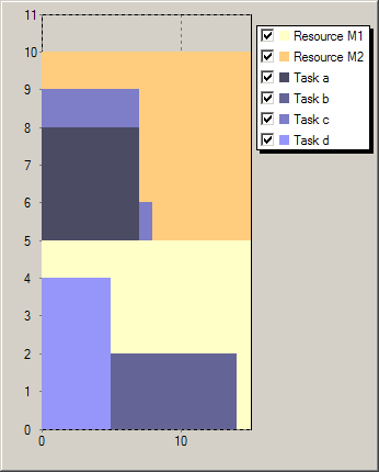
Results
Figure Solutions for scheduling with resource choice shows two solutions generated by the execution of our model. The first solution uses a lesser total amount resource but the second one is optimal with respect to the objective of minimizing the makespan.
 |
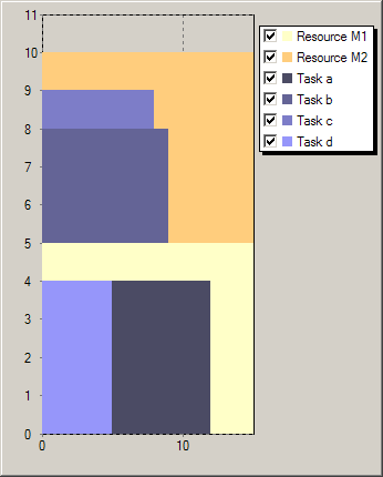 |
Figure 5.5: Solutions for scheduling with resource choice
Note: leaving the decision about the resource choice open for the solver considerably increases the complexity of a scheduling problem. We therefore recommend to use this feature sparingly. Optimization problems involving resource assignment and sequencing aspects are often more easily solved by a decompostion approach (see the Xpress Whitepaper Hybrid MIP/CP solving with Xpress Optimizer and Xpress Kalis).
Resource profiles
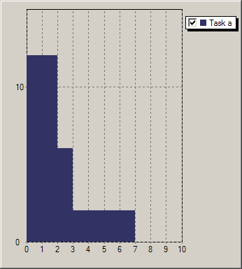
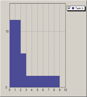
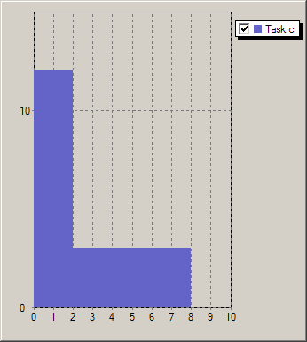
In all preceding examples we have worked with the assumption that a task is defined by a constant, though not necessarily fixed resource requirement (respectively resource provision, consumption, or production). Following this line of thought, a sequence of processesing steps with different resource usages would be represented by a corresponding number of tasks, each with a constant resource usage. However, the number of cptask objects required by such a formulation may be prohibitively large. Kalis therefore offers the possibility to define profiled tasks, that is, tasks with a non-constant resource usage profile. A task resource usage profile states for every time unit of the execution of the task the corresponding amount of resource. For example the four tasks in Figure Task profiles have the profiles Profilea: (12, 12, 6, 2, 2, 2, 2), Profileb: (12, 12, 6, 2, 2, 2, 2, 2, 2), Profilec: (12, 12, 3, 3, 3, 3, 3, 3), and Profiled: (6, 6, 6, 6, 6) respectively.
 |
 |
 |
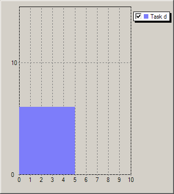 |
Figure 5.6: Task profiles
Model formulation
Let TASKS = {'a','b','c','d'} be the set of tasks and res a resource of capacity CAP required by all tasks for their execution. With the objective of minimizing the makespan of the schedule we may formulate the model as follows.
tasks taskj (j ∈ TASKS)
minimize makespan
res.capacity = CAP
∀ j ∈ TASKS: taskj.start,taskj.end ∈ {0,...,HORIZON}
∀ j ∈ TASKS: taskj.duration = DURj
∀ j ∈ TASKS: taskj.requirementres = Profilej
This model formulation differs from a standard cumulative scheduling model (see Section Cumulative scheduling: discrete resources only in a single point: the resource requirement Profilej of a task j is a list of values and not just a single constant.
Implementation
Let us now take a look at the model formulation with Mosel.
 uses "kalis"

 setparam("KALIS_DEFAULT_LB", 0)

 forward procedure print_solution

 declarations
  TASKS = {"a","b","c","d"}           ! Index set of tasks
  Profile: array(TASKS) of list of integer   ! Task profiles
  DUR: array(TASKS) of integer        ! Durations of tasks

  task: array(TASKS) of cptask        ! Tasks
  res: cpresource                     ! Cumulative resource
 end-declarations

 DUR::(["a","b","c","d"])[7, 9, 8, 5]
 Profile("a"):= [12, 12, 6, 2, 2, 2, 2]
 Profile("b"):= [12, 12, 6, 2, 2, 2, 2, 2, 2]
 Profile("c"):= [12, 12, 3, 3, 3, 3, 3, 3]
 Profile("d"):= [6, 6, 6, 6, 6]

! Define a discrete resource
 set_resource_attributes(res, KALIS_DISCRETE_RESOURCE, 18)
 res.name:="machine"

! Define tasks with profiled resource usage
 forall(t in TASKS) do
  task(t).duration:= DUR(t)
  task(t).name:= t
  requires(task(t), resusage(res, Profile(t)))
 end-do

 cp_set_solution_callback(->print_solution)
 starttime:=timestamp

! Solve the problem
 if cp_schedule(getmakespan)=0 then
  writeln("No solution")
  exit(0)
 end-if

! Solution printing
 writeln("Schedule with makespan ", getsol(getmakespan), ":")
 forall(t in TASKS)
  writeln(t, ": ", getsol(getstart(task(t))), " - ", getsol(getend(task(t))))

! ****************************************************************

! Print solutions during enumeration at the node where they are found.
! 'getrequirement' can only be used here to access solution information,
! not after the enumeration (it returns a value corresponding to the
! current state, that is, 0 after the enumeration).
 procedure print_solution
  writeln(timestamp-starttime, "sec. Solution: ", getsol(getmakespan))

  forall(i in 0..getsol(getmakespan)-1) do
   write(strfmt(i,2), ": ")
   forall(t in TASKS | getrequirement(task(t), res, i)>0)
    write(t, ":", getrequirement(task(t), res, i), "  " )
   writeln("(total ", sum(t in TASKS) getrequirement(task(t), res, i), ")")
  end-do
 end-procedure

end-model
The statement of the resource constraints (requires) uses an additional type of scheduling object for the definition of the resource profiles, namely resusage. We have already encountered this object in Section Alternative resources where it was employed in the definition of sets of alternative resources. In the present case there is only a single resource that must be used by all tasks, we now employ resusage to define resource usage profiles.
Results
The chart in Figure Solution for scheduling with resource profile shows an optimal schedule of the four tasks on a resource with capacity 18. All tasks are completed by time 11.

Figure 5.7: Solution for scheduling with resource profile
Resource idle times and preemption of tasks
In the examples of cumulative scheduling we have looked at so far resources are defined with a fixed constant capacity. In reality, it often happens that the resource availability is not constant over time: a resource 'staff', for instance, is likely to show variations corresponding to the presence or absence of personnel. Such changes to the resource level can be defined periodwise with the subroutine setcapacity. In the case of machine resources there may be scheduled downtimes for maintenance or other breaks, such as week-ends, relating to working hours. Any such periods that are known from the outset should be marked as 'unavailable for processing tasks'.
From the perspective of tasks there are two cases of resource unavailability: (1) any task starting before the resource unavailability must also be finished before the begin of this period (generally known as non-preemptive scheduling), and (2) a task started before the unavailability resumes its processing once the resource becomes available again (the case of preemptive scheduling).
With Kalis, the first case applies when resource capacities are set to 0 using setcapacity (independent of the type of the task). The second case is modeled by using profiled tasks and indicating resource unavailability with setidletimes.
For simplicity's sake, we merely consider two tasks, a and b, that are to be scheduled on a resource of capacity 3 that is unavailable in certain time periods. Task a has a constant resource requirement of 1 for 4 units of time, task b has the resource usage profile (1,1,1,2,2,2,1,1). Both tasks are preemptive.
Model formulation
Let TASKS = {'a','b'} be the set of tasks and res a resource of capacity CAP required by the tasks for their execution. The set IDLESET contains the time periods during which the resource is unavailable preempting the processing of tasks. With the objective of minimizing the makespan of the schedule we may formulate the model as follows.
tasks taskj (j ∈ TASKS)
minimize makespan
res.capacity = CAP
res.idletimes = IDLESET
∀ j ∈ TASKS: taskj.start,taskj.end ∈ {0,...,HORIZON}
∀ j ∈ TASKS: taskj.duration ≥ DURj
∀ j ∈ TASKS: taskj.requirementres = Profilej
Please notice that we do not fix the durations of the tasks in this formulation: we may indicate (lower or upper) bounds to restrict the total duration of a task, but if we want to leave room for preemptions the bounds on the durations of tasks must include some slack.
Implementation
The following model shows how to implement our example problem with Mosel.
model "Preemption"
 uses "kalis", "mmsystem"

 setparam("KALIS_DEFAULT_LB", 0)

 forward procedure print_solution

 declarations
  aprofile,bprofile: list of integer
  a,b: cptask
  res: cpresource
 end-declarations

! Define a discrete resource
 set_resource_attributes(res, KALIS_DISCRETE_RESOURCE, 3)

! Create a 'hole' in the availability of the resource:
! Uncomment one of the following two lines to compare their effect
! setcapacity(res, 1, 2, 0);  setcapacity(res, 7, 8, 0)
 setidletimes(res, (1..2)+(7..8))

! Define two tasks (a: constant resource use, b: resource profile)
 a.duration >= 4
 a.name:= "task_a"
 aprofile:= [1,1,1,1]

 b.duration >= 8
 b.name:= "task_b"
 bprofile:= [1,1,1,2,2,2,1,1]

! Resource usage constraints
 requires(a, resusage(res,aprofile))
 requires(b, resusage(res,bprofile))

 cp_set_solution_callback(->print_solution)

! Solve the problem
 if cp_schedule(getmakespan)<>0 then
  cp_show_sol
 else
  writeln("No solution")
 end-if

! ****************************************************************

 procedure print_solution
  writeln("Solution: ", getsol(getmakespan))
  writeln("Schedule: a: ", getsol(getstart(a)), "-", getsol(getend(a))-1,
          ", b: ", getsol(getstart(b)), "-", getsol(getend(b))-1)
  writeln("Resource usage:")
  forall(t in 0..getsol(getmakespan)-1)
   writeln(formattext("%5d: Cap: %d, a:%d, b:%d", t, getcapacity(res,t),
           getrequirement(a, res, t), getrequirement(b, res, t)) )
 end-procedure

end-model
There are several equivalent ways of stating the constant resource usage of task a. Instead of defining explicitly the complete profile we may simply write
requires(a, resusage(res,1))
or even shorter:
requires(a, 1, res)
Results
The model shown above produces the following solution output.
Solution: 12
Schedule: a: 0-5, b: 0-11
Resource usage:
    0: Cap: 3, a:1, b:1
    1: Cap: 3, a:0, b:0
    2: Cap: 3, a:0, b:0
    3: Cap: 3, a:1, b:1
    4: Cap: 3, a:1, b:1
    5: Cap: 3, a:1, b:2
    6: Cap: 3, a:0, b:2
    7: Cap: 3, a:0, b:0
    8: Cap: 3, a:0, b:0
    9: Cap: 3, a:0, b:2
   10: Cap: 3, a:0, b:1
   11: Cap: 3, a:0, b:1
The same model, replacing the line
setidletimes(res, (1..2)+(7..8))
by this version indicating non-preemptive resource unavailability
setcapacity(res, 1, 2, 0); setcapacity(res, 7, 8, 0)
results in the following solution where the tasks are placed in such a way that they do not overlap with any 'hole' in resource availability.
Solution: 17
Schedule: a: 3-6, b: 9-16
Resource usage:
    0: Cap: 3, a:0, b:0
    1: Cap: 0, a:0, b:0
    2: Cap: 0, a:0, b:0
    3: Cap: 3, a:1, b:0
    4: Cap: 3, a:1, b:0
    5: Cap: 3, a:1, b:0
    6: Cap: 3, a:1, b:0
    7: Cap: 0, a:0, b:0
    8: Cap: 0, a:0, b:0
    9: Cap: 3, a:0, b:1
   10: Cap: 3, a:0, b:1
   11: Cap: 3, a:0, b:1
   12: Cap: 3, a:0, b:2
   13: Cap: 3, a:0, b:2
   14: Cap: 3, a:0, b:2
   15: Cap: 3, a:0, b:1
   16: Cap: 3, a:0, b:1
It is also possible to define both, preemptive and non-preemptive times of unavailability for the same resource. For example, if times 1-2 correspond to a weekend where products may remain on the machine R and times 7-8 are required for maintenance operations during which the machine must imperatively be empty we would state in our model:
 setidletimes(res, 1, 2, 0)
 setcapacity(res, (7..8))
In this case the execution of task a may start at time 0, whereas task b will again be processed in times 9-16.
Enumeration
In the previous scheduling examples we have used the default enumeration for scheduling problems, invoked by the optimization function cp_schedule. The built-in search strategies used by the solver in this case are particularly suited if we wish to minimize the completion time of a schedule. With other objectives the built-in strategies may not be a good choice, especially if the model contains decision variables that are not part of scheduling objects (the built-in strategies always enumerate first the scheduling objects) or if we wish to maximize an objective. kalis makes it therefore possible to use the standard optimization functions cp_minimize and cp_maximize in models that contain scheduling objects, the default search strategies employed by these optimization functions being different from the scheduling-specific ones. In addition, the user may also define his own problem-specific enumeration as shown in the following examples.
User-defined enumeration strategies for scheduling problems may take two different forms: variable-based and task-based. The former case is the subject of Chapter Enumeration, and we only give a small example here (Section Variable-based enumeration). The latter will be explained with some more detail by the means of a job-shop scheduling example.
Variable-based enumeration
When studying the problem solving statistics for the bin packing problem in Section Cumulative scheduling: discrete resources we find that the enumeration using the default scheduling search strategies requires several hundred nodes to prove optimality. With a problem-specific search strategy we may be able to do better! Indeed, we shall see that a greedy-type strategy, assigning the largest files first, to the first disk with sufficient space is clearly more efficient.
Using cp_minimize
The only decisions to make in this problem are the assignments of files to disks, that is, choosing a value for the start time variables of the tasks. The following lines of Mosel code order the tasks in decreasing order of file sizes and define an enumeration strategy for their start times assigning each the smallest possible disk number first. Notice that the sorting subroutine qsort is defined by the module mmsystem that needs to be loaded with a uses statement at the beginning of the model.
 declarations
  Strategy: array(range) of cpbranching
  FSORT: array(FILES) of integer
 end-declarations

 qsort(SYS_DOWN, SIZE, FSORT)       ! Sort files in decreasing order of size
 forall(f in FILES)
  Strategy(f):=assign_var(KALIS_SMALLEST_MIN, KALIS_MIN_TO_MAX,
                          {getstart(file(FSORT(f)))})
 cp_set_branching(Strategy)

 if not cp_minimize(diskuse) then writeln("Problem infeasible"); end-if
The choice of the variable selection criterion (first argument of assign_var) is not really important here since every strategy Strategyf only applies to a single variable and hence no selection takes place. Equivalently, we may have written
 declarations
  Strategy: cpbranching
  FSORT: array(FILES) of integer
  LS: cpvarlist
 end-declarations

 qsort(SYS_DOWN, SIZE, FSORT)       ! Sort files in decreasing order of size
 forall(f in FILES)
  LS+=getstart(file(FSORT(f)))
 Strategy:=assign_var(KALIS_INPUT_ORDER, KALIS_MIN_TO_MAX, LS)
 cp_set_branching(Strategy)

 if not cp_minimize(diskuse) then writeln("Problem infeasible"); end-if
With this search strategy the first solution found uses 3 disks, that is, we immediately find an optimal solution. The whole search terminates after 17 nodes and takes only a fraction of the time needed by the default scheduling or minimization strategies.
Using cp_schedule
The scheduling search consists of a pretreatment (shaving) phase and two main phases (KALIS_INITIAL_SOLUTION and KALIS_OPTIMAL_SOLUTION) for which the user may specify enumeration strategies by calling cp_set_schedule_search with the corresponding phase selection. The `initial solution' phase aims at providing quickly a good solution whereas the `optimal solution' phase proves optimality. Any search limits such as maximum number of nodes apply separately to each phase, an overall time limit (parameter KALIS_MAX_COMPUTATION_TIME) only applies to the last phase.
The definition of variable-based branching schemes for the scheduling search is done in exactly the same way as what we have seen previously for standard search with cp_minimize or cp_maximize, replacing cp_set_strategy by cp_set_schedule_strategy:
 cp_set_schedule_branching(KALIS_INITIAL_SOLUTION, Strategy)
 if cp_schedule(diskuse)=0 then writeln("Problem infeasible"); end-if
With this search strategy, the optimal solution is found in the 'initial solution' phase after just 8 nodes and the enumeration stops there since the pretreatment phase has proven a lower bound of 3 which is just the value of the optimal solution.
NB: to obtain an output log from the different phases of the scheduling search set the control parameter KALIS_VERBOSE_LEVEL to 2, that is, add the following line to your model before the start of the solution algorithm.
setparam("KALIS_VERBOSE_LEVEL", 2)
Task-based enumeration
A task-based enumeration strategy consists in the definition of a selection strategy choosing the task to be enumerated, a value selection heuristic for the task durations, and a value selection heuristic for the task start times.
Consider the typical definition of a job-shop scheduling problem: we are given a set of jobs that each need to be processed in a fixed order by a given set of machines. A machine executes one job at a time. The durations of the production tasks (= processing of a job on a machine) and the sequence of machines per job for a 6×6 instance are shown in Table 66 job-shop instance from . The objective is to minimize the makespan (latest completion time) of the schedule.
| Job | Machines | Durations | ||||||||||
|---|---|---|---|---|---|---|---|---|---|---|---|---|
| 1 | 3 | 1 | 2 | 4 | 6 | 5 | 1 | 3 | 6 | 7 | 3 | 6 |
| 2 | 2 | 3 | 5 | 6 | 1 | 4 | 8 | 5 | 10 | 10 | 10 | 4 |
| 3 | 3 | 4 | 6 | 1 | 2 | 5 | 5 | 4 | 8 | 9 | 1 | 7 |
| 4 | 2 | 1 | 3 | 4 | 5 | 6 | 5 | 5 | 5 | 3 | 8 | 9 |
| 5 | 3 | 2 | 5 | 6 | 1 | 4 | 9 | 3 | 5 | 4 | 3 | 1 |
| 6 | 2 | 4 | 6 | 1 | 5 | 3 | 3 | 3 | 9 | 10 | 4 | 1 |
Model formulation
Let JOBS denote the set of jobs and MACH (MACH = {1,...,NM}) the set of machines. Every job j is produced as a sequence of tasks taskjm where taskjm needs to be finished before taskj,m+1 can start. A task taskjm is processed by the machine RESjm and has a fixed duration DURjm.
The following model formulates the job-shop scheduling problem.
tasks taskjm (j ∈ JOBS, m ∈ MACH)
minimize finish
finish = maximumj ∈ JOBS(taskj,NM.end)
∀ m ∈ MACH: resm.capacity = 1
∀ j ∈ JOBS, m ∈ MACH: taskjm.start, taskjm.end ∈ {0,...,MAXTIME}
∀ j ∈ JOBS, m ∈ {1,...,NM-1}: taskjm.successors = {taskj,m+1}
∀ j ∈ JOBS, m ∈ MACH: taskjm.duration = DURjm
∀ j ∈ JOBS, m ∈ MACH: taskjm.requirementRESjm = 1
Implementation
The following Mosel model implements the job-shop scheduling problem and defines a task-based branching strategy for solving it. We select the task that has the smallest remaining domain for its start variable and enumerate the possible values for this variable starting with the smallest. A task-based branching strategy is defined with the kalis function task_serialize, that takes as arguments the user task selection, value selection strategies for the duration and start variables, and the set of tasks it applies to. Such task-based branching strategies can be combined freely with any variable-based branching strategies.
model "Job shop (CP)"
 uses "kalis", "mmsystem"

 parameters
  DATAFILE = "jobshop.dat"
  NJ = 6                                 ! Number of jobs
  NM = 6                                 ! Number of resources
 end-parameters

 forward function select_task(tlist: cptasklist): integer

 declarations
  JOBS = 1..NJ                           ! Set of jobs
  MACH = 1..NM                           ! Set of resources
  RES: array(JOBS,MACH) of integer       ! Resource use of tasks
  DUR: array(JOBS,MACH) of integer       ! Durations of tasks

  res: array(MACH) of cpresource         ! Resources
  task: array(JOBS,MACH) of cptask       ! Tasks
 end-declarations

 initializations from "Data/"+DATAFILE
  RES DUR
 end-initializations

 HORIZON:= sum(j in JOBS, m in MACH) DUR(j,m)
 forall(j in JOBS) getend(task(j,NM)) <= HORIZON

! Setting up the resources (capacity 1)
 forall(m in MACH)
  set_resource_attributes(res(m), KALIS_UNARY_RESOURCE, 1)

! Setting up the tasks (durations, resource used)
 forall(j in JOBS, m in MACH)
  set_task_attributes(task(j,m), DUR(j,m), res(RES(j,m)))

! Precedence constraints between the tasks of every job
 forall (j in JOBS, m in 1..NM-1)
!  getstart(task(j,m)) + DUR(j,m) <= getstart(task(j,m+1))
  setsuccessors(task(j,m), {task(j,m+1)})

! Branching strategy
 Strategy:=task_serialize(->select_task, KALIS_MIN_TO_MAX,
            KALIS_MIN_TO_MAX,
            union(j in JOBS, m in MACH | exists(task(j,m))) {task(j,m)})
 cp_set_branching(Strategy)

! Solve the problem
 starttime:= gettime

 if not cp_minimize(getmakespan) then
  writeln("Problem is infeasible")
  exit(1)
 end-if

! Solution printing
 cp_show_stats
 write(gettime-starttime, "sec ")
 writeln("Total completion time: ", getsol(getmakespan))
 forall(j in JOBS) do
  write("Job ", strfmt(j,-2))
  forall(m in MACH | exists(task(j,m)))
   write(formattext("%3d:%3d-%2d", RES(j,m), getsol(getstart(task(j,m))),
         getsol(getend(task(j,m)))))
  writeln
 end-do

!*******************************************************************
! Task selection for branching
 function select_task(tlist: cptasklist): integer
  declarations
   Tset: set of integer
  end-declarations

 ! Get the number of elements of "tlist"
  listsize:= getsize(tlist)

 ! Set of uninstantiated tasks
  forall(i in 1..listsize)
   if not is_fixed(getstart(gettask(tlist,i))) then
    Tset+= {i}
   end-if

  returned:= 0

  ! Get a task with smallest start time domain
  smin:= min(j in Tset) getsize(getstart(gettask(tlist,j)))
  forall(j in Tset)
   if getsize(getstart(gettask(tlist,j))) = smin then
    returned:=j; break
   end-if

 end-function

end-model
Results
An optimal solution to this problem has a makespan of 55. In comparison with the default scheduling strategy, our branching strategy reduces the number of nodes that are enumerated from over 300 to just 105 nodes with a comparable model execution time (however, for larger instances the default scheduling strategy is likely to outperform our branching strategy). The default minimization strategy does not find any solution for this problem within several minutes running time.

Figure 5.8: Solution graph
Alternative search strategies
Similarly to what we have seen above, we may define a user task selection strategy for the scheduling search. The only modifications required in our model are to replace cp_set_branching by cp_set_schedule_strategy and cp_minimize by cp_schedule. The definition of the user task choice function select_task remains unchanged.
! Branching strategy
 Strategy:=task_serialize(->select_task, KALIS_MIN_TO_MAX,
            KALIS_MIN_TO_MAX,
            union(j in JOBS, m in MACH | exists(task(j,m))) {task(j,m)})
 cp_set_schedule_strategy(KALIS_INITIAL_SOLUTION, Strategy)

! Solve the problem
 if cp_schedule(getmakespan)=0 then
  writeln("Problem is infeasible")
  exit(1)
 end-if
This strategy takes even fewer nodes for completing the enumeration than the standard search with user task selection.
Instead of the user-defined task selection function select_task it is equally possible to use one of the predefined task selection criteria:
- KALIS_SMALLEST_EST / KALIS_LARGEST_EST
- choose task with the smallest/largest lower bound on its start time ( 'earliest start time'),
- KALIS_SMALLEST_LST / KALIS_LARGEST_LST
- choose task with the smallest/largest upper bound on its start time ( 'latest start time'),
- KALIS_SMALLEST_ECT / KALIS_LARGEST_ECT
- choose task with the smallest/largest lower bound on its completion time ( 'earliest completion time'),
- KALIS_SMALLEST_LCT / KALIS_LARGEST_LCT
- choose task with the smallest/largest upper bound on its completion time ( 'latest completion time').
 Strategy:=task_serialize(KALIS_SMALLEST_LCT, KALIS_MIN_TO_MAX,
            KALIS_MIN_TO_MAX,
            union(j in JOBS, m in MACH | exists(task(j,m))) {task(j,m)})
Even more specialized task selection strategies can be defined with the help of group_serialize. In this case you may decide freely which are the variables to enumerate for a task and in which order they are to be considered. The scope of group_serialize is not limited to tasks, you may use this subroutine to define search strategies involving other types of (user) objects.
Choice of the propagation algorithm
The performance of search algorithms for scheduling problems relies not alone on the definition of the enumeration strategy; the choice of the propagation algorithm for resource constraints may also have a noticeable impact. The propagation type is set by an optional last argument of the procedure set_resources_attributes, such as
set_resource_attributes(res, KALIS_DISCRETE_RESOURCE, CAP, ALG)
where ALG is the propagation algorithm choice.
For unary resources we have a choice between the algorithms KALIS_TASK_INTERVALS and KALIS_DISJUNCTIONS. The former achieves stronger pruning at the cost of a larger computational overhead making the choice of KALIS_DISJUNCTIONS more competitive for small to medium sized problems. Taking the example of the jobshop problem from the previous section, when using KALIS_DISJUNCTIONS the default scheduling search is about 4 times faster than with KALIS_TASK_INTERVALS although the number of nodes explored is slightly larger than with the latter.
The propagation algorithm options for cumulative resources are KALIS_TASK_INTERVALS and KALIS_TIMETABLING. The filtering algorithm KALIS_TASK_INTERVALS is stronger and relatively slow making it the preferred choice for hard, medium-sized problems whereas KALIS_TIMETABLING should be given preference for very large problems where the computational overhead of the former may be prohibitive. In terms of an example, the binpacking problem we have worked with in Sections Cumulative scheduling: discrete resources and Variable-based enumeration solves about three times faster with KALIS_TASK_INTERVALS than with KALIS_TIMETABLING (using the default scheduling search).
© 2001-2025 Fair Isaac Corporation. All rights reserved. This documentation is the property of Fair Isaac Corporation (“FICO”). Receipt or possession of this documentation does not convey rights to disclose, reproduce, make derivative works, use, or allow others to use it except solely for internal evaluation purposes to determine whether to purchase a license to the software described in this documentation, or as otherwise set forth in a written software license agreement between you and FICO (or a FICO affiliate). Use of this documentation and the software described in it must conform strictly to the foregoing permitted uses, and no other use is permitted.