Linear and Mixed Integer Linear Programming Software: A Guide to Its Applications, Benefits, and Business Impact

Key Takeaways:

• Linear and mixed integer linear programming (LP and MILP) are business-critical decision tools, not mathematical abstractions. Supply chain planning, energy dispatch, and workforce scheduling involve interdependencies across cost, capacity, service levels, and timing that cannot be resolved manually at operational scale. Linear and mixed integer linear programming provides a rigorous framework that delivers economically defensible, repeatable decisions, making them foundational to operational performance rather than incidental to it.
• MILP is the dominant enterprise optimization formulation because most high-value decisions require either a mix of either continuous and discrete decisions or purely discrete decisions. Enterprise operational decisions span fundamentally different variable types. Production volumes are continuous, machine activation is binary and facility selection is discrete. Mixed-integer linear programming consolidates all of these within a single formulation, making it the standard for production planning, logistics network design, and workforce optimization. 
• Solver performance in production is not equivalent to solver performance on a benchmark. Enterprise optimization demands consistent re-optimization at scale as demand, supply, asset availability, and business rules shift continuously. For operations teams across transportation, energy, and retail environments, sustained throughput and planning responsiveness under production conditions are the primary determinants of operational value. 
• Linear and mixed integer linear programming are the prescriptive layers that convert data into operational decisions. Predictive models estimate demand, lead times, and failure risk but fail to determine the appropriate course of action. Linear and mixed integer linear programming bridges that gap by converting data and predictions into concrete, defensible decisions on order fulfillment, inventory allocation, vehicle routing, and more.
• FICO^® Xpress Optimization sets the performance and deployment standard for enterprise linear and mixed integer linear programming. Its MILP solver has delivered up to 5.7x performance improvements since 2020 with advanced presolve, parallel processing, and cutting-plane techniques built for large-scale  MILP problems. FICO Xpress supports APIs for Python, C, C++, Java, and .NET and provides governance, explainability and version control capabilities that enable optimization models to be deployed, maintained and scaled across enterprise functions. 

What Is Linear Programming?

Linear programming is a mathematical optimization method used to allocate limited resources across competing activities while maximizing or minimizing a linear objective function with decisions that can take continuous, fractional values. 

It applies when all decision variables are continuous, and the objective and constraints can all be expressed as linear functions, which makes the technique especially valuable for structured planning and operational decision-making. 

Linear programming is widely deployed across supply chain, transportation, energy, retail, and e-commerce environments, where resource constraints and competing priorities demand precise and calculable answers. 

The standard linear programming formulation consists of:

• Decision variables with optional upper and lower bounds 
• An objective function
• A set of equality or inequality constraints that define the feasible region

Consider a small conceptual example. A farmer needs to determine how much wheat and corn to plant on his or her 50 acres of land. Both wheat and corn have a market price, a per-acre expected yield, and a per-acre labor cost. The market prices for each crop and per-acre expected yields and labor costs are known or predicted values that the optimization model incorporates into the decision model.

The question the farmer needs to determine is, “How should the 50 acres of land be allocated between corn and wheat production to maximize total profit?”

Contained in that question are three unknowns:

1. How many acres of wheat should be planted?
2. How many acres of corn should be planted?
3. Which combination maximizes expected profit?

Questions 1. and 2. are answered through the decision variables in the optimization model. Since both decision variables (i.e., the number of acres to plant wheat and the number of acres to plant corn) are allowed to take fractional values, these are continuous decision variables. For example, planting 31.2 acres of wheat and 18.8 acres of corn is a plausible, feasible solution, but is it the optimal one that maximizes total profit?

Question 3. defines the objective function. Using the input data and decision variables, the objective function is a linear function constructed to find the optimal acre allocation for both corn and wheat that maximizes the farmer’s total expected profit.

Lastly, constraints are used to ensure the model adheres to specific business rules. One of those constraints for this model is ensuring the total number of acres doesn’t exceed the total capacity of 50 acres.

Once the model is constructed, a solver then searches that feasible region to identify the optimal solution by using algorithms such as the simplex or interior-point methods. The practical value of linear programming extends beyond theory, because modern optimization software can embed these models within decision management and prescriptive analytics workflows. Solving a linear programming problem (e.g., a linear relaxation) is also the first step to solving a mixed integer programming model.

What is Mixed Integer Linear Programming?

Mixed Integer Linear Programming (MILP), often reduced to Mixed Integer Programming (MIP) for short, combines continuous and integer variables in one model, allowing a wider range of real-world decisions to be represented in a unified framework. In production planning, output volumes may be continuous while machine activation is modeled as binary. MILP remains the dominant enterprise optimization formulation because most business problems require both variable types to capture operational constraints and decision logic accurately. 

However, MILP problems are more complex to solve. A common way solvers manage this complexity is by first solving the MILP as a linear programming problem, then progressively narrowing the search until the best integer-feasible solution is found. This requires relaxing the integer and discrete variables and running a linear programming model first before the integer and/or binary decisions can be found. 

In certain special cases, the structure of the optimization problem is strong enough that the simpler linear programming model naturally produces integer or binary decisions without requiring the full MILP search process. When this happens, the model can often be solved faster and at larger scale using linear programming alone. Minimum Cost Network Flow (see the example below) is a classic example. Due to its special network structure, the linear programming formulation  produces the same integer flow decisions that would otherwise require a MILP formulation.

What Makes an Infeasible Model?

In some cases you will have an LP or MILP model for which no solution satisfies all constraints at the same time, usually because some constraints are mutually contradictory. Infeasibility analysis helps practitioners identify conflicting constraints and determine whether the formulation or the underlying data must be revised before the model can be solved. 

For example, consider a price optimization model seeking to find the optimal prices of four products: Apples, Bananas, Coconuts, and Dragon Fruit, and you impose the following business rules as constraints into the model:

• The price of Apples must be greater than the price of Bananas (A >= B)
• The price of Bananas must be greater than the price of Coconuts (B >= C)
• The price of Coconuts must be greater than the price of Apples (C >= A)

Clearly these three rules cannot coexist together as they are logically impossible for the optimization model to adhere to. Representing these, among other pricing rules, as a network, they form a directed cycle (A --> B, B --> C, C --> A). The presence of these three constraints will make the model infeasible, and is just one example of what can cause a model to be infeasible.

Business Problems Represented as LP and MILP Models

Deterministic 

The examples below are popular business problems that are solved using linear and mixed-integer linear programming, but are far from an exhaustive list. The flexibility of these optimization modeling techniques are what make them so applicable across nearly every industry.

Transportation Models

This specialized class of linear programs optimizes the flow of goods or resources from supply nodes to demand nodes, usually to minimize total transportation cost. These models support network design, distribution planning, and last-mile logistics decisions. They also often serve as one component within broader supply chain optimization formulations. 

Consider an example called the Traveling Salesman Problem. The Traveling Salesman Problem seeks to find the shortest or lowest-cost route for visiting each location in a network exactly once and returning to the starting point. It is easy to understand but difficult to solve at scale without optimization because the number of possible routes grows extremely quickly as more locations are added. 

For example, the network below shows a greenway network with all routes connecting 11 parks. 

The objective of the Traveling Salesman Problem is to find the minimum cost tour, or a cycle that traverses only a subset of routes that visits each park once while minimizing total distance. 

The result returns the optimal subset that visits each of the 11 parks and minimizes total distance to 34 units.

Assignment Models

Assignment models allocate resources to tasks on a one-to-one basis. Each resource is assigned to exactly one task, and each task is covered by at most one resource. Common applications include assigning aircraft to routes, workers to shifts, and vehicles to delivery zones. The Linear Assignment Problem is a classic example that uses linear programming to produce binary decisions (e.g., assign player i to team j) due to the special properties of its design.

Suppose you need to assign workers to tasks. In the example below, six workers need to be assigned to six of eight total tasks based on worker preferences (ranked from 1-8 based on individual preference). 1 indicates a worker’s most desired preference. 2 indicates a worker’s second most desired preference, and so on.

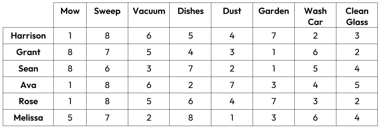
The objective is to assign one worker to one task that minimizes the sum of all preference weights. A worker can be assigned to only one task, and a task can be assigned to at most one worker.

For this particular example, since there are two more tasks than workers, two tasks will go unassigned. 

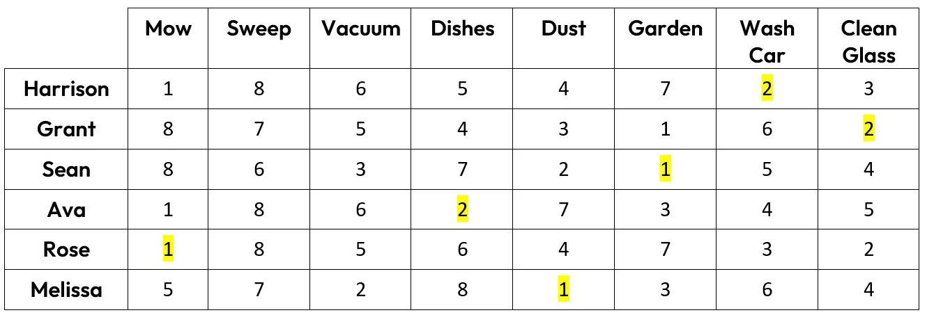
The optimal assignments are highlighted in yellow, with a total objective value minimized at 9. The tasks ‘Sweep’ and ‘Vacuum’ went unassigned. 

Blending Models

Blending models determine the optimal mix of input ingredients or components to produce an output that satisfies defined cost, quality, or composition requirements. These models are widely used in food and beverage manufacturing, refining, and chemical production. In these settings, the objective is typically to minimize input cost while meeting minimum or maximum thresholds for each attribute of the finished product. 

Network Flow Models

Network flow models optimize the flow of goods, energy, or capacity through a connected system of nodes and arcs, subject to capacity constraints, flow conservation at each node, and costs on each arc. These models generalize both transportation and assignment problems. They are used across logistics networks, utility grids, and telecommunications infrastructure. The Minimum Cost Network Flow model referenced above is one of many transportation model examples that leverages linear programming.

Consider a simple distribution network with two facilities, one distribution center, and two warehouses. Facilities are supply nodes, warehouses demand nodes, and the distribution center is a transshipment node, meaning it serves as simply a passthrough for flow along the network. 

Each route segment (arc) has an associated cost per unit and maximum allowable capacity. 

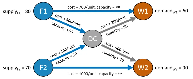
The objective is to determine how to transport product (flow) through the network to meet warehouse demand at the minimum total cost. 

Using linear programming, the optimal solution can be quickly found and returned. In this example, total cost is minimized at $107,000.

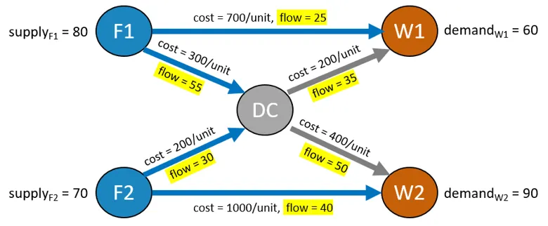
Even with small examples like this one, finding the optimal solution manually is a nontrivial exercise. However, the true power of linear and mixed integer linear programming is when these problems are solved at scale on commercial-sized instances.

Why Are LP and MILP Models Essential for Business Optimization?

Most meaningful business decisions come down to allocating limited resources (budget, inventory, staff hours, transportation capacity) in a way that satisfies competing constraints while achieving a clear objective, often minimizing cost or meeting distribution targets. 

As the number of variables and constraints grows, these problems quickly exceed what a person can reason through with a spreadsheet or a set of rules of thumb. Linear programming addresses this by translating the decision into a mathematical model: an objective function to optimize, subject to a system of linear constraints. Because the underlying mathematics guarantees that the solution found is truly optimal (not just a reasonable guess), organizations can trust that linear optimization gets them the best possible answer given the stated assumptions. 

Linear programming is especially important as businesses scale. A transportation network with a handful of routes might be manageable through manual planning, but a national distribution system with thousands of origin-destination pairs, capacity limits, and delivery windows is not. Linear programming scales gracefully to these larger problems, handling thousands or even millions of variables and constraints without losing rigor. It also brings consistency: the same model applied to similar situations will produce comparable, defensible decisions, whereas ad hoc or heuristic approaches tend to drift and produce uneven results as conditions change. 

How Do Linear and Mixed Integer Programming Solve Complex Optimization Problems?

Step 1: Define the Structured Mathematical Model 

Linear and mixed integer programming begins by converting a real-world business problem into a structured mathematical model by:

• Identifying decision variables: the core quantities the model seeks to determine such as shipment quantities or inventory positions.
• Constructing a linear objective function: the primary performance goal. Typical objectives include minimizing total cost, maximizing profit margin, or reducing transit time.
• Defining a set of linear constraints that represent the operational environment limits, such as capacity ceilings or demand requirements. 

Step 2: Define the Algorithm Model and Structure 

• Defining a feasible region, the set of all solutions that simultaneously satisfy every constraint. This region serves as the solution space within which the solver searches for the optimal outcome.
• Applying the algorithms: optimization software applies one or more algorithms to navigate the feasible region efficiently. Commonly used methods include the simplex algorithm, the barrier method and interior-point algorithms, each suited to different model characteristics.
• Validating assumptions and data quality: before results can be acted upon, users must validate underlying assumptions, verify data quality, and confirm that model coefficients accurately reflect operational reality.

Step 3: Analysis and Decision

• Analyzing post-solve data: extract deeper insight from the solution to reveal which constraints are binding, quantify the economic value of relaxing those constraints, and identify where incremental changes would deliver the greatest benefit. 
• Making the optimal decision: linear programming is an end-to-end decision optimization process. Once the exact combination of variable values has been solved, the resulting solution can be used as the provably optimal choice among all feasible options giving decision-makers a concrete, defensible decision.

Step 4: Deploy and Manage the Model with DecisionOps

• De-risking model rollout: confirm the model’s performance from local development to staging and production environments before deploying the model live. Implement CI/CD (Continuous Integration and Continuous Delivery/Deployment) to initiate testing workflows that validate acceptance criteria such as business KPIs, explore “what if” scenarios to understand the impact input data and configuration changes will have on model output, and run a candidate model in shadow mode before promoting it.
• Deploying the model to production: integrate the model into existing production systems as a service (via API), account for scalable compute, and stay agile with simple rollbacks that point to a fallback version in case of a production failure.
• Managing and observing models: manage model versions and configurations across environments in a space that’s accessible to teammates, audit all decisions via a managed system of record, see a changelog of all model updates (and who made them), and troubleshoot issues quickly with logs and metadata for every model run.

How Are Businesses Using Linear and Mixed Integer Linear Programming to Solve Real-World Business Problems?

Linear programming is used in business operations to balance cost, capacity, service levels, and execution speed. The examples below show how linear programming, supported by FICO^® Xpress Optimization, delivers measurable value at production scale.

Manufacturing and Production Planning

Manufacturing teams must decide production mix, machine scheduling, raw material allocation, and labor deployment. These choices affect unit cost, throughput, service levels, and margin. Linear programming models these trade-offs through objective functions and resource constraints, then identifies a plan that minimizes cost or maximizes output while meeting capacity, labor, material, and delivery requirements.

PepsiCo has used FICO Xpress Optimization since 2009 for production planning across its global manufacturing network. Its implementation includes a mixed integer programming model with up to 600,000 decision variables and up to 400,000 constraints. Reported outcomes include:

• A 30% reduction in daily production model solve times was achieved through the systematic application of Xpress solver tuning controls.
• An immediate 15% reduction in solve time was achieved after upgrading to a newer Xpress release, with no model changes.
• Production scheduling was deployed globally across all manufacturing sites, including 36 sites in the United States and Canada.
• Between 400 and 500 production planning instances were executed per day across multiple planning horizons.
• Reduction of staffing plan creation time from two to three days per department to less than five minutes for 80% of instances and less than one hour for all instances.

Lirthik Durai, Principal Scientist of Optimization at PepsiCo, stated: “With Xpress, we can go from an idea to a working proof of concept in days, not months. That speed is what gets people excited about using optimization.”

Energy Generation and Grid Dispatch

Energy generation and grid dispatch are established applications of linear and mixed integer programming. Generation commitment aligns asset choice, output, and scheduling with demand and constraints such as ramp rates, minimum up/down times, transmission limits, and fuel costs.

AFRY has integrated FICO Xpress Optimization in its BID3 power market modeling platform. The platform applies linear and mixed integer programming to represent energy system characteristics, fuel price dynamics, and market design mechanisms. Its objective is to compute least-cost outcomes across multiple geographies and planning horizons at the scale required for policy analysis and investment planning. 

Reported results include:

• BID3 serves 30 organizations worldwide and informs billion-dollar energy investment decisions across major European markets, including the United Kingdom, Norway, Germany, and Denmark
• In 2025, AFRY reported a 25% increase in BID3’s global user base, supported by enhanced modeling capabilities enabled by FICO Xpress
• The platform supports major national policy studies, including the United Kingdom’s 2038 to 2043 Carbon Budget analysis
• ENTSO-E used BID3 for its Bidding Zone Review to assess electricity bidding zone configurations across Europe in support of efficient market operation and renewable integration

Zeid Munir, Principal of Modeling Solutions at AFRY, explained the selection rationale: “We chose FICO’s optimization solution for its industrial-grade linear and mixed-integer programming capabilities and scalability across complex, multi-dimensional problems. No other solution on the market provided the tools we need.”

Supply Chain and Logistics Network Optimization

Supply chain and logistics are mature linear programming applications, requiring optimization of transportation, inventory, warehouse capacity, sourcing and service levels across multi-echelon networks. Solving these decisions in isolation often creates avoidable inefficiencies. Linear programming allows the network to be modeled as a single optimization problem against a global objective.

In practice, this means identifying the least-cost or highest-service allocation of supply, inventory, and fulfillment decisions while respecting lead times, facility capacities, route limitations and contractual constraints. For leaders responsible for distribution, transportation, retail, or ecommerce operations, solver speed, model scalability, and implementation reliability directly affect performance.

For example, DoorDash relies on FICO® Xpress Optimization at the core of its real-time Dasher dispatch system, improving delivery matching speed by 10–100x over its previous approach. As Sifeng Lin, Operations Research Scientist at DoorDash, put it: "FICO Xpress plays a critical role in DoorDash's central real-time Dasher dispatch system. It solves our large-scale MIP problem optimally in seconds and has been completely reliable since implementation."

Workforce Scheduling and Headcount Optimization

Workforce scheduling is another domain in which linear programming delivers direct operational value. Organizations in manufacturing, retail, healthcare, and distribution must align staffing levels with demand while accounting for worker qualifications, shift requirements, labor regulations, service-level targets and attrition assumptions. In these environments, the difference between heuristic scheduling and mathematically optimized planning is frequently evident in labor cost, fill rates, overtime, and retention.

For example, at the start of the 2020 pandemic, Boeing’s crew solution team used its market-leading Jeppesen digital aviation software to solve a crucial nurse scheduling problem for the intensive care unit (ICU) for Karolinska University Hospital in Stockholm, Sweden’s second largest hospital. Using Jeppesen Crew Rostering, which employs FICO Xpress Optimization, Boeing created rosters for over 300 nurses and healthcare workers during the peak period, resulting in more workable shifts for staff and better coverage for the hospital. 

“The biggest challenge, by far, was time,” said Daniel Roth, Senior Business Advisor with Boeing. “We only had a week to produce the initial schedule, which had to incorporate who could work when, individual nurse competences, special requirements with respect to their schedules, and other factors. This data was not available in a structured way, but rather in the heads of current schedulers and management. Fortunately, our extensively used aviation solution with FICO Xpress Optimization as an integral part, enables an end-user to quickly build schedules.”

Across these use cases, the pattern is the same: competing objectives, binding constraints, and decision spaces too large for manual evaluation. Linear programming provides the modeling framework, while optimization software delivers the performance needed for reliable production use. 

Why Is Linear and Mixed Integer Programming Central to AI and Decision Management Workflows?

Linear and Mixed Integer Programming Both Solve a Different Problem Than Predictive Models

Predictive models estimate outcomes, while linear and mixed integer programming turns forecasts such as demand, lead times, and failure risk into feasible, optimal decisions under resource constraints and business objectives. In enterprise settings, high-value decisions require allocating shared capacity under constraints. Inventory positioning, order prioritization, and production-distribution planning require methods that balance competing objectives; forecasting alone is not enough.

Connecting Forecasting to Operational Execution

Linear programming links analytical output to operational decisions and supports re-optimization as conditions change. When demand shifts, linear programming determines how to reallocate inventory, adjust facility loading, and quantify cost-service trade-offs. As forecasts and constraints change, models are re-solved for scenario analysis and near-real-time replanning. In supply chain, transportation, energy, retail and e-commerce, narrow planning windows make continuous, governed re-optimization an operational requirement, not just an analytical option.

For a concrete example showing how to combine probabilistic forecasting with FICO Xpress’s linear programming solver, read this recent blog post by FICO Xpress and PyMC.

Transparency That Supports Governance and Executive Adoption

Linear programming models are fully inspectable: variables capture business decisions, constraints encode policies, and objective coefficients make priorities explicit. This transparency makes validation, executive review, and deployment oversight easier. Where explainability, auditability, and policy alignment are required, this structural clarity is operationally important and often determines enterprise-scale adoption and governance of optimization models.

A Foundational Layer in Modern Decision Intelligence Stacks

Linear programming is neither a legacy method nor simply a complement to machine learning. It is the layer that converts predictive output into governed, economically aligned operational decisions. For organizations building decision intelligence capabilities across supply chain, operations, energy or retail, linear programming provides the mathematical framework that makes prescriptive analytics repeatable, scalable and operationally defensible.

What Distinguishes FICO Xpress Optimization as the Leading Linear Programming Software?

Solver Performance for Demanding Models

FICO Xpress delivers linear programming and MILP performance aimed at the issues technical buyers usually evaluate first: 

• Solve speed on large models
• Stability on numerically difficult formulations
• Ability to sustain throughput in production rather than only in benchmark-style runs 

For teams managing network design, production planning, routing, inventory or workforce models, that matters because the bottleneck is often not model formulation alone, but how quickly and reliably the solver can re-optimize as inputs change. 

FICO Xpress is built for that operating reality. Its MIP solver has delivered performance improvements of up to 5.7x since 2020, indicating continued investment in core algorithmic performance across product releases rather than one-time gains.

Modeling Flexibility Across Implementation Paths

FICO Xpress supports multiple implementation languages including Python, C, C++, Java, and .NET, which is important for organizations that need to fit optimization into existing engineering and analytics environments. 

In practice, this gives teams flexibility in how they deploy models: researchers can prototype in Python, while enterprise development teams can integrate the same optimization logic into larger applications, services or planning systems in the language stack already used internally. 

For teams comparing linear programming tools or commercial solvers, this reduces a common implementation risk: having a strong solver that requires disruptive changes to the surrounding architecture.

Enterprise Deployment Readiness

For most enterprises, solver quality is only part of the evaluation. The larger question is whether optimization can be governed, explained, deployed, and maintained at scale across business functions. 

FICO Xpress addresses that broader production requirement with support for governance, version control, explainability and production orchestration. Xpress’s deployment capabilities are relevant when optimization moves from analyst-owned models to operational systems that influence recurring decisions, service levels, cost structures, and compliance-sensitive processes. 

Industry Fit and Operational Context

FICO Xpress is particularly relevant in industries where optimization is not an occasional analytical exercise but a continuous operational requirement. In supply chain, transportation, energy, retail and ecommerce, decision models are frequently re-run as demand shifts, constraints tighten, asset availability changes, and service targets need to be maintained. 

These environments typically combine large model sizes with narrow decision windows, which makes solver speed, scalability, and implementation reliability central selection criteria. FICO Xpress aligns well with those requirements because it is positioned for repeated re-optimization under production conditions, where consistency and turnaround time matter as much as raw mathematical capability.

Case Study in Deployment: Shell

Shell, working with FICO and Yokogawa, deployed FICO Xpress within its Platform for Advanced Control and Estimation (PACE), showing how the solver can be embedded in industrial optimization environments where decisions must connect directly to plant operations. 

The deployment optimized control processes across LNG, GTL, and chemical plants worldwide. Shell reported reduced process variability, increased throughput and improved operational reliability. The same deployment also supports decarbonization objectives by optimizing energy consumption and reducing greenhouse gas emissions at industrial scale, which is often a key requirement when optimization investments must support both operational and environmental performance.

FICO Xpress as a Foundation for Prescriptive Analytics

For leaders evaluating linear programming software as part of a broader decision management or prescriptive analytics stack, FICO Xpress offers more than a standalone optimization engine. It combines solver performance for linear programming and MILP, flexibility across implementation languages, and the governance features needed to operationalize models in enterprise settings. 

That combination is especially relevant for organizations trying to move from isolated optimization studies to durable decision systems that can be deployed, monitored and improved over time. As a result, FICO Xpress is better understood less as a solver for individual models and more as a platform component for sustained decision optimization at business scale.

Learn More About FICO Xpress Optimization Capabilities

• Download our PepsiCo case study to see how one of the world's largest food and beverage manufacturers reduced production planning solve times by 30%, cut workforce planning from days to minutes, and executed 400–500 daily optimization instances across 36 global manufacturing sites using FICO Xpress Optimization. 
• Download our FICO Xpress Solver solution sheet to learn how Xpress delivers industry-leading LP, MILP and nonlinear solver performance for supply chain, energy, manufacturing and retail applications. It helped one airline save $49 million annually, enabled a food manufacturer to save $35 million through production and transportation optimization and helped an energy company cut CO2 emissions by 20–50 million metric tons annually. 
• Request your complimentary 60-day FICO Xpress trial to assess solver performance on your own LP and MILP models and evaluate how Xpress maintains throughput and planning responsiveness at production scale. 
• Our FICO Xpress Solver eBook for Energy and Utilitiescovers how optimization is applied across the energy lifecycle, from generation dispatch and grid balancing to refinery scheduling and distribution planning, with proven results including Shell's plant-wide control optimization across hundreds of global processing sites and Artelys securing power supply for over 300 million Europeans. 
• Explore FICO Xpress Optimization to learn how a single platform combines LP and MILP solver performance, multi-language deployment flexibility and enterprise governance to support repeatable decision optimization across supply chain, manufacturing, energy, and retail operations.